Building a Variational Autoencoder with TensorFlow: A Practical Guide

Master the fundamentals of autoencoders, discover how variational autoencoders enhance them, and walk through a step‑by‑step TensorFlow implementation.

Artificial intelligence has reshaped countless sectors, and data compression is no exception. Autoencoders—especially their variational variants—provide powerful, generative compression schemes that are both efficient and expressive. This guide breaks down the core concepts and walks you through a full TensorFlow implementation using the MNIST dataset.

Autoencoder Applications

Autoencoders are widely adopted in fields ranging from neural machine translation to drug discovery, image denoising, and anomaly detection. Their ability to learn compressed, informative representations makes them a go‑to tool for modern ML pipelines.

Key Components of an Autoencoder

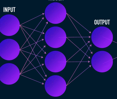
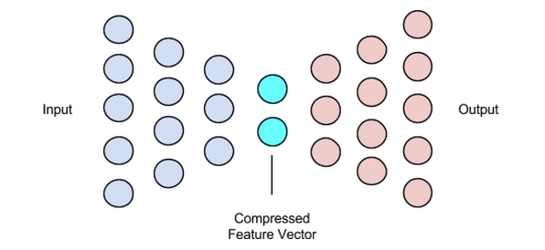
Unlike typical neural networks, autoencoders feature a bottleneck that forces a low‑dimensional latent representation. The architecture comprises three primary parts:

• Encoder – compresses input data into a latent vector.
• Bottleneck (Latent Vector) – stores the most salient features.
• Decoder – reconstructs the input from the latent vector.

The encoder and decoder are usually feed‑forward networks, but specialized variants—convolutional for images, recurrent for text—are common in practice.

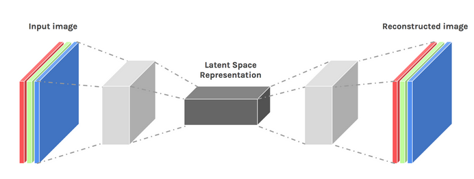
Encoder

The encoder maps high‑dimensional inputs (e.g., 28×28 pixel images) to a compact latent vector. During training, it optimizes its weights so the latent vector captures essential information, enabling the decoder to reconstruct the input with minimal loss.

Bottleneck (Latent Vector)

The latent vector size is a trade‑off: too small and you lose critical detail; too large and you undermine compression and inflate computation. Selecting an appropriate dimensionality is crucial for model performance.

Decoder

The decoder is a mirror of the encoder, transforming the latent vector back into the original data space. It typically uses transposed convolutions or upsampling layers to recover spatial resolution.

Training Autoencoders

Autoencoders are trained end‑to‑end using gradient‑based optimizers like Adam. The objective is to minimize a reconstruction loss that quantifies the discrepancy between the input and its reconstruction.

Loss Functions

Common choices include L1, L2, and mean squared error (MSE). Each measures how close the output is to the input, making them suitable for generative reconstruction tasks.

Network Variants

While multi‑layer perceptrons (MLPs) can serve as encoders/decoders, convolutional neural networks (CNNs) are preferred for image data due to their spatial awareness. Recurrent networks excel with sequential data such as text.

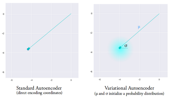
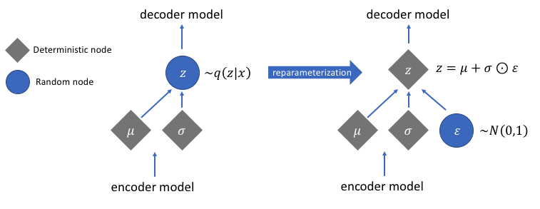
Standard autoencoders lack creativity—they can only reproduce data seen during training. Introducing stochasticity via a variational framework unlocks generative capabilities.

Variational Autoencoders (VAEs)

VAEs modify the standard architecture in two ways:

• The encoder outputs a mean vector and a variance vector, defining a Gaussian distribution.
• A Kullback‑Leibler (KL) divergence term is added to the loss to regularize the latent distribution toward a unit Gaussian.

During inference, the encoder samples a latent vector from the learned distribution, enabling the decoder to generate diverse, realistic reconstructions. This stochasticity mitigates the discontinuities often observed in deterministic autoencoders.

TensorFlow Implementation

Below is a concise, production‑ready TensorFlow implementation of a convolutional VAE trained on MNIST.

Data Preparation

(train_images, _), (test_images, _) = tf.keras.datasets.mnist.load_data()
train_images = train_images.reshape(-1, 28, 28, 1).astype('float32')
test_images = test_images.reshape(-1, 28, 28, 1).astype('float32')

train_images /= 255.
test_images /= 255.

train_images[train_images >= .5] = 1.
train_images[train_images < .5] = 0.

test_images[test_images >= .5] = 1.
test_images[test_images < .5] = 0.

TRAIN_BUF = 60000
BATCH_SIZE = 100
TEST_BUF = 10000
train_dataset = tf.data.Dataset.from_tensor_slices(train_images).shuffle(TRAIN_BUF).batch(BATCH_SIZE)
test_dataset = tf.data.Dataset.from_tensor_slices(test_images).shuffle(TEST_BUF).batch(BATCH_SIZE)

VAE Model Definition

class CVAE(tf.keras.Model):
    def __init__(self, latent_dim):
        super(CVAE, self).__init__()
        self.latent_dim = latent_dim
        self.inference_net = tf.keras.Sequential([
            tf.keras.layers.InputLayer(input_shape=(28, 28, 1)),
            tf.keras.layers.Conv2D(32, 3, strides=2, activation='relu'),
            tf.keras.layers.Conv2D(64, 3, strides=2, activation='relu'),
            tf.keras.layers.Flatten(),
            tf.keras.layers.Dense(latent_dim + latent_dim),  # mean & logvar
        ])
        self.generative_net = tf.keras.Sequential([
            tf.keras.layers.InputLayer(input_shape=(latent_dim,)),
            tf.keras.layers.Dense(7*7*32, activation='relu'),
            tf.keras.layers.Reshape((7, 7, 32)),
            tf.keras.layers.Conv2DTranspose(64, 3, strides=2, padding='SAME', activation='relu'),
            tf.keras.layers.Conv2DTranspose(32, 3, strides=2, padding='SAME', activation='relu'),
            tf.keras.layers.Conv2DTranspose(1, 3, padding='SAME'),  # logits
        ])

    @tf.function
    def sample(self, eps=None):
        if eps is None:
            eps = tf.random.normal(shape=(100, self.latent_dim))
        return self.decode(eps, apply_sigmoid=True)

    def encode(self, x):
        mean, logvar = tf.split(self.inference_net(x), num_or_size_splits=2, axis=1)
        return mean, logvar

    def reparameterize(self, mean, logvar):
        eps = tf.random.normal(shape=mean.shape)
        return eps * tf.exp(logvar * .5) + mean

    def decode(self, z, apply_sigmoid=False):
        logits = self.generative_net(z)
        if apply_sigmoid:
            return tf.sigmoid(logits)
        return logits

Key helper functions—encode, reparameterize, and decode—encapsulate the VAE workflow. The reparameterize method implements the reparameterization trick, enabling gradient flow through stochastic sampling.

Reparameterization Trick

Sampling a latent vector directly from a distribution breaks differentiability. By expressing the sample as z = mean + std * eps where eps ~ N(0,1), gradients propagate through mean and std. The KL divergence term further aligns the learned distribution with a standard normal, promoting smooth latent spaces.

Quick Summary of Steps

1. Define encoder and decoder architectures.
2. Implement the reparameterization trick to enable back‑propagation.
3. Train the model end‑to‑end, minimizing reconstruction loss plus KL divergence.

For the full code and additional training scripts, visit the TensorFlow official tutorial.

Image credit: Chiman Kwan (modified)