Linearizing Resistive Sensor Bridges with Two Proven Hardware Methods

Measuring minuscule resistance changes in sensors can be daunting. This article presents two hardware techniques that eliminate bridge non‑linearity errors, improving accuracy and calibration simplicity.

The resistance of a resistive sensor changes in response to a physical variable such as temperature or force. The percentage change is typically tiny – for instance, a strain gauge may vary by less than 1 % over its entire range.

Accurate measurement of such small changes demands a highly precise circuit. Bridge configurations make this easier, but even a linear sensor can produce a non‑linear bridge output.

Software or hardware methods can correct this non‑linearity. Below, we explore two proven hardware approaches.

Bridge Non‑linearity of Resistive Sensors

Consider a pressure sensor with a linear response:

R_sensor = R₀ + Mx

Assuming the slope M equals the initial resistance R₀, the response simplifies to R₀(1 + x).

Using a standard bridge (Figure 1), where the other three resistors equal R₀, maximizes sensitivity. The bridge output is:

V_out = V_r \(\left(\dfrac{R_0(1+x)}{R_0+R_0(1+x)} - \dfrac{1}{2}\right)\)

which reduces to

V_out = V_r \(\dfrac{x}{2(2+x)}\)  (Equation 1)

Because the relationship is non‑linear, for small x (x ≪ 2) we can approximate:

V_out ≈ V_r \(\dfrac{x}{4}\)  (Equation 2)

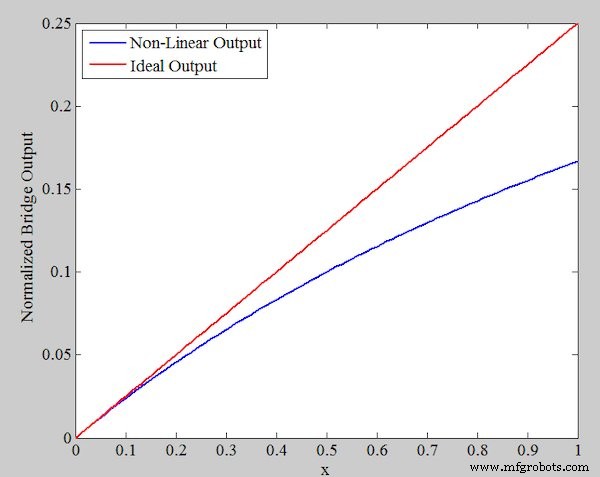
Figure 2 shows the normalized output $V_{out}/V_{r}$ for both equations, illustrating how deviation grows with x.

Quantifying Non‑linearity Error

Rewriting Equation 1:

V_out = V_r \(\dfrac{x}{4}\) \(\dfrac{1}{1 + \dfrac{x}{2}}\)

Assuming $x/2 \ll 1$, a Taylor expansion gives:

V_out ≈ V_r \(\dfrac{x}{4}\) (1 – \(\dfrac{x}{2}\))

Comparing with Equation 2, the absolute non‑linearity error is

E_{Non‑Linearity} = V_r \(\dfrac{x}{4}\) \(\dfrac{x}{2}\)

Expressed as a percentage of the ideal value:

Percentage Error = \(\dfrac{x}{2} \times 100\%\)

Example

For a sensor with R₀ = 100 Ω and maximum x = 0.01, the peak linearity error is

Percentage Error = \(\dfrac{0.01}{2} \times 100\% = 0.5\%\)

While software compensation is possible, a linear bridge output directly improves measurement precision and eases calibration.

Method 1: Voltage Proportional to Resistance Change

Figure 3 illustrates the first linearization circuit.

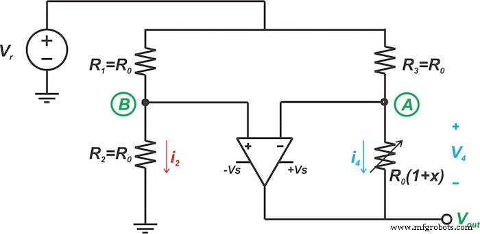
By forcing a constant reference current $I_{Ref}$ through the sensor (Figure 4), the sensor voltage becomes

V_sensor = I_Ref · R₀(1 + x)

Rearranged:

V_sensor = R₀ I_Ref + R₀ I_Ref x

The first term is constant; the second is linear in x. The op‑amp in Figure 3 keeps node B at $V_{r}/2$, forcing a constant current $V_{r}/(2R_{0})$ through the sensor. Consequently, the output is

V_out = -\(\dfrac{V_{r}}{2}\) x

which is a clean linear function of x.

Method 2: Current Proportional to Resistance Change

Figure 5 presents the second approach.

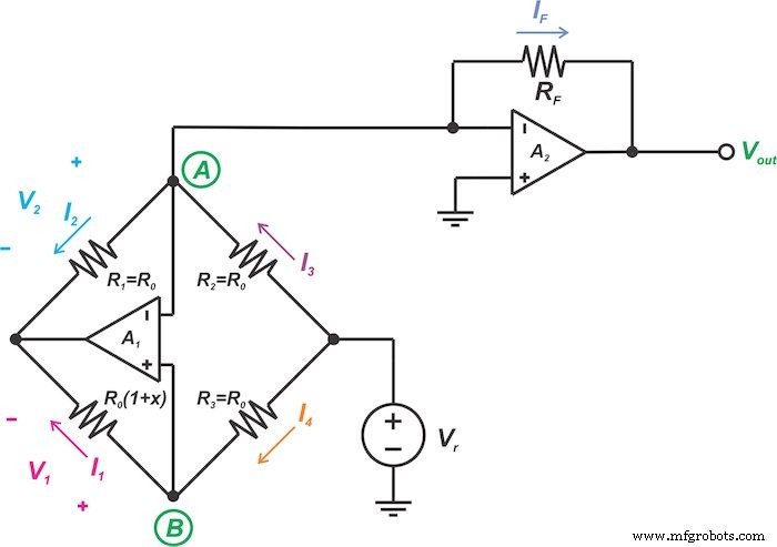
In this design, branch 1 carries a current proportional to the sensor resistance:

I₁ = I_Ref · R₀(1 + x)

Branch 2 supplies a constant current $I_{Ref} R_{0}$, so the differential current in branch 3 is $I_{Ref} R_{0} x$. Using two op‑amps with identical inputs, the circuit subtracts the constant term and outputs

V_out = V_r \(\dfrac{R_{F}}{R_{0}}\) x

Choosing the ratio $R_{F}/R_{0}$ allows arbitrary gain. Although this method requires an extra op‑amp, it offers flexible scaling.

---

To explore more in‑depth articles, please visit my article list.