SPICE Diode Modeling: A Practical Guide to Accurate Simulation

SPICE is the industry‑standard for circuit simulation, and diodes are one of its most frequently modeled components. A diode’s behaviour is captured in SPICE through two statements: the device element and the model definition. The element statement connects the diode to the circuit, while the model statement specifies its electrical characteristics.

Defining a Diode in SPICE

Every diode element must start with the letter d followed by an optional identifier (e.g., d1, dtest, d101). The next two numbers are the anode and cathode node numbers. The final token is the name of the model that will be defined later.

Example:

    d1 1 2 mod1

The corresponding model statement starts with .model, followed by the model name, the keyword d, and then optional parameter assignments in the form Parameter=Value. Parameters that are omitted default to values shown in the tables below.

Example:

    .model mod1 d

Example with parameters:

    D2 1 2 Da1N4004
    .model Da1N4004 D (IS=18.8n RS=0 BV=400 IBV=5.00u CJO=30 M=0.333 N=2)

Key Diode Parameters

Symbol	Name	Parameter	Units	Default
IS	IS	Saturation current (diode equation)	A	1E‑14
RS	RS	Parasitic resistance (series resistance)	Ω	0
n	N	Emission coefficient, 1 to 2	-	1
τD	TT	Transit time	s	0
CD(0)	CJO	Zero‑bias junction capacitance	F	0
ϕ0	VJ	Junction potential	V	1
m	M	Junction grading coefficient	-	0.5
Eg	EG	Activation energy (eV)	-	1.11
pi	XTI	IS temperature exponent	-	3.0
kf	KF	Flicker noise coefficient	-	0
af	AF	Flicker noise exponent	-	1
FC	FC	Forward bias depletion capacitance coefficient	-	0.5
BV	BV	Reverse breakdown voltage	V	∞
IBV	IBV	Reverse breakdown current	A	1E‑3

Getting a Reliable Model

The most accurate way to obtain a SPICE model is to download it directly from the manufacturer’s website. If that is unavailable, you can construct a model from the datasheet by extracting the key parameters listed above. As a third option, you can measure the device yourself and fit the SPICE parameters to the measured I‑V curve.

Parameter Extraction Example – 1N4004

To illustrate the process, we’ll derive a model for the common 1N4004 rectifier. We start by selecting an emission coefficient N of 2.0, which is typical for silicon rectifiers. Using the diode equation

I_D = I_S (e^{V_D/(N V_T)} - 1)

and the datasheet point (V_D = 0.925 V at I_D = 1 A, V_T = 26 mV at 25 °C) we solve for I_S:

I_S = 18.8 nA

Other parameters are set to their default values unless the datasheet specifies otherwise:

• RS = 0 Ω (initially, later adjusted for better fit)
• TT = 0 s (no Q_RR data available)
• CJO = 30 pF (from V_R‑C_J graph)
• M = 0.333 (linearly graded junction)
• VJ = 1 V, EG = 1.11 eV, XTI = 3.0
• BV = 400 V, IBV = 5 µA (reverse‑breakdown specs)

Resulting model statement:

.model Da1N4004 D (IS=18.8n RS=0 BV=400 IBV=5.00u CJO=30 +M=0.333 N=2.0 TT=0)

Fine‑Tuning the Model

When comparing the derived model to the manufacturer’s model and the datasheet I‑V curve, we noticed that the current at 1.4 V exceeded the spec (12 A). Adjusting the series resistance to 28.6 mΩ brought the curve into alignment at 1.4 V while maintaining the 1 A point. Further fine‑tuning can be achieved by iterating N and RS until the simulated curve matches the datasheet curve across the full range.

Comparing Models

The following SPICE circuit demonstrates the three models in parallel for easy comparison:

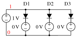SPICE circuit for comparing manufacturer, datasheet‑derived, and default models.

Netlist excerpt:

*SPICE circuit <03468.eps> from XCircuit v3.20
D1 1 5 DI1N4004
V1 5 0 0
D2 1 3 Da1N4004
V2 3 0 0
D3 1 4 Default
V3 4 0 0
V4 1 0 1
.DC V4 0 1400mV 0.2m
.MODEL Da1N4004 D (IS=18.8n RS=28.6m BV=400 IBV=5.00u CJO=30 +M=0.333 N=2.0 TT=0)
.MODEL DI1N4004 D (IS=76.9n RS=42.0m BV=400 IBV=5.00u CJO=39.8p +M=0.333 N=1.45 TT=4.32u)
.MODEL Default D
.END

Zener, Tunnel, and Gunn Diodes

For Zener diodes, two modeling strategies exist:

• Set the BV parameter to the Zener voltage (e.g., .model D1N4469 D (BV=15 IBV=17m)). This is the simplest approach.
• Use a subcircuit with a diode clamper that forces the breakdown voltage (see the subcircuit below for a 1N4477A model).

Example subcircuit:

.SUBCKT DI-1N4744A 1 2
* Terminals A K
D1 1 2 DF
DZ 3 1 DR
VZ 2 3 13.7
.MODEL DF D (IS=27.5p RS=0.620 N=1.10 +CJO=78.3p VJ=1.00 M=0.330 TT=50.1n)
.MODEL DR D (IS=5.49f RS=0.804 N=1.77)
.END

For tunnel diodes, a pair of JFETs can emulate the negative differential resistance region, as shown in reference [KHM]. Similarly, a Gunn diode can be modeled with two JFETs to capture its microwave oscillation behavior ([ISG]).

Key Takeaways

• Use the diode element to connect the device; the .model statement defines its electrical behavior.
• Static parameters (N, IS, RS) dominate low‑frequency performance; reverse‑breakdown specs (BV, IBV) matter for high‑voltage applications.
• Dynamic behavior hinges on TT and CJO; include them for accurate transient simulations.
• Manufacturer‑supplied models are preferred; if unavailable, derive from datasheet data or empirical measurements.