From Vacuum Tubes to Integrated Circuits: The Evolution of Operational Amplifier Models

When most people think of operational amplifiers, they imagine silicon‑based ICs. However, the earliest commercial op‑amps were vacuum‑tube circuits.

In 1952, George A. Philbrick Researches, Inc. introduced the K2‑W, the first general‑purpose op‑amp. It featured two twin‑triode tubes housed in an octal (8‑pin) socket, making it easy to install and service in the chassis of the era.

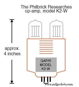
The schematic shows the twin‑triode assembly alongside ten resistors and two capacitors – a remarkably simple design for its time.

How Vacuum Tubes Operate

Vacuum tubes behave like N‑channel depletion‑type IGFETs: the control grid conducts more current when it is more positive relative to the cathode, and less when it is less positive. In the K2‑W, the left twin‑triode forms a differential pair that converts the inverting and non‑inverting inputs into a single amplified signal. A 1 MΩ – 2.2 MΩ voltage divider feeds this signal to the left triode of the second tube, which provides additional voltage gain and inverts the output. The second triode then drives a non‑inverting stage for current gain. Neon glow tubes act as voltage regulators, similar to zener diodes, supplying bias voltage between the two single‑ended amplifiers.

With a dual supply of +300 / –300 V, the K2‑W could swing its output only ±50 V. It offered an open‑loop gain of 15 000 – 20 000, a slew rate of ±12 V/µs, a maximum output current of 1 mA, and quiescent power consumption exceeding 3 W (not counting filament power). In 1952 dollars, it cost about $24.

Solid‑State Transistors and the Next Generation

Transistor technology enabled op‑amps that consumed far less quiescent power and were far more reliable, while maintaining comparable performance. Philbrick’s 1966 P55A, for instance, featured an open‑loop gain of 40 000, a slew rate of 1.5 V/µs, and an output swing of ±11 V from a ±15 V supply. Its maximum output current was 2.2 mA, and it sold for $49 (about $21 for the utility grade). The P55A was a discrete‑component design housed in a solid “brick” that resembled a large IC package.

It is possible to build a basic op‑amp from discrete parts, as illustrated by the schematic below. The differential pair formed by transistors Q3 and Q4 serves the same role as the twin‑triode in the K2‑W, converting differential inputs into a single‑ended output.

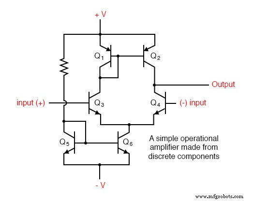
A simple operational amplifier constructed from discrete components.

Integrated‑Circuit Revolution

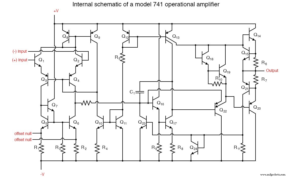
The introduction of ICs in the mid‑1960s transformed op‑amp design. Fairchild released the 702, 709, and the now‑iconic 741 between 1964 and 1968. Although the 741 is considered obsolete by today’s standards, it remains popular among hobbyists for its robustness and short‑circuit protection.

Internal schematic of a 741 op‑amp.

With SSI technology, the 741 contains only a handful of components, making it impractical to replicate with discrete parts. This illustrates the clear advantages of even the earliest ICs over large discrete‑component assemblies.

Performance Comparison of Popular Op‑amps

Below is a selection of low‑cost op‑amps that illustrate the range of performance characteristics available today. The 741 is included as a benchmark, though newer designs far exceed its specifications.

Widely used operational amplifiers

Model	Devices / Package	Power Supply (V)	Bandwidth (MHz)	Bias Current (nA)	Slew Rate (V/µS)	Output Current (mA)
TL082	2	12 / 36	4	8	13	17
LM301A	1	10 / 36	1	250	0.5	25
LM318	1	10 / 40	15	500	70	20
LM324	4	3 / 32	1	45	0.25	20
LF353	2	12 / 36	4	8	13	20
LF356	1	10 / 36	5	8	12	25
LF411	1	10 / 36	4	20	15	25
741C	1	10 / 36	1	500	0.5	25
LM833	2	10 / 36	15	1050	7	40
LM1458	2	6 / 36	1	800	10	45
CA3130	1	5 / 16	15	0.05	10	20

As the table shows, bias current varies dramatically: the CA3130, a MOSFET‑based design, delivers an astonishing 0.05 nA (50 pA) bias current, while the LM833, which uses bipolar transistors, can draw over 1 µA. The CA3130’s input impedance is advertised as 1.5 TΩ (1.5 × 10¹² Ω).

Although the 741 is a staple in textbooks, its performance has been eclipsed by modern devices. For instance, the LM1458 shares the 741’s package but offers a wider supply range, a 50‑fold higher slew rate, and almost twice the output current, all while retaining short‑circuit protection.

Here are my recommendations:

• Low‑bias‑current circuits (e.g., low‑speed integrators): CA3130.
• General‑purpose DC amplification: LM1458 (two op‑amps in one 8‑pin DIP).
• Higher bandwidth: LF353 (JFET input, four‑times the bandwidth of the LM1458).
• Low‑voltage operation: LM324 (runs on as little as 3 V, offers four op‑amps in a 14‑pin package).
• High‑frequency AC amplification: LM318.

High‑Bandwidth and High‑Current Op‑amps

Special‑purpose op‑amps deliver exceptional performance at modest cost. The following tables highlight models optimized for bandwidth or current output.

High‑bandwidth operational amplifiers

Model	Devices / Package	Power Supply (V)	Bandwidth (MHz)	Bias Current (nA)	Slew Rate (V/µS)	Output Current (mA)
CLC404	1	10 / 14	232	44 000	2600	70
CLC425	1	5 / 14	1900	40 000	350	90

The CLC404 costs $21.80, comparable to the price of the original K2‑W in 1952 dollars. The CLC425 is more affordable at $3.23 per unit. Both achieve high speed at the expense of higher bias current and tighter supply ranges.

High‑current operational amplifiers

Model	Devices / Package	Power Supply (V)	Bandwidth (MHz)	Bias Current (nA)	Slew Rate (V/µS)	Output Current (mA)
LM12CL	1	15 / 80	0.7	1000	9	13 000
LM7171	1	5.5 / 36	200	12 000	4100	100

The LM12CL can deliver a staggering 13 A of output current at a price of $14.40. In contrast, the LM7171 offers a high slew rate (4 kV/µs) for only $1.19.

For designs that demand extreme precision or repeatability, manufacturers such as Burr‑Brown and Analog Devices provide pre‑engineered instrumentation amplifiers and other specialized devices. Although these blocks are pricier than bare op‑amps, they simplify circuit design and often improve reliability.

RELATED WORKSHEET:

• Basic Operational Amplifiers Worksheet