The Operational Amplifier: Foundations, Features, and Key Applications

Before digital electronics, computers performed calculations by translating numbers into voltages and currents. By using resistive voltage dividers and amplifiers, basic arithmetic operations—division and multiplication—could be carried out on these analog signals. This approach proved especially valuable for simulating physical systems, where a variable voltage might represent a physical quantity such as velocity or force.

Using the Derivative Function to Compute Capacitor Current

Capacitors and inductors possess reactive properties that naturally model calculus relationships. The current through a capacitor equals the time‑rate of change of its voltage—its derivative. If we let the voltage across a capacitor represent an object’s velocity, then the resulting current corresponds to the force required to accelerate or decelerate that object, with the capacitance acting as the object’s mass:

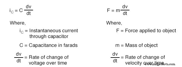
This analog computation of the derivative—known as differentiation—is performed automatically by a capacitor without any “programming” required, offering a simple, low‑cost method for simulating differential equations.

Because analog circuits are inexpensive and easier to construct than complex mechanical models, they were widely adopted in the early research and development of mechanical systems. High‑accuracy, easily configurable amplifiers were essential to achieve realistic simulations.

Why Differential Amplifiers Outperform Single‑Ended Designs

Early analog computers revealed that differential amplifiers with extremely high voltage gain delivered the required accuracy and configurability better than custom‑gain single‑ended amplifiers. By attaching simple external components to the high‑gain differential amplifier’s inputs and output, virtually any gain or function could be obtained without modifying the internal circuitry. These high‑gain differential amplifiers became known as operational amplifiers (op‑amps) due to their pivotal role in analog computer mathematics.

Key Features of Modern Op‑amps

• High Input Impedance: The 741, for example, draws a maximum of 0.5 µA, and field‑effect input stages can draw even less.
• Low Output Impedance: Typically around 75 Ω for the 741, with many models offering built‑in short‑circuit protection.
• DC and AC Performance: Direct coupling allows amplification of DC signals, while bandwidth limits define the maximum voltage‑rise time.
• Cost‑Effective: A single integrated circuit provides performance that would otherwise require a complex discrete‑transistor amplifier, unless extremely high power is needed.

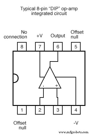
Figure 1 shows the pinout for a single 741 op‑amp in an 8‑pin DIP package. Dual and quad packages, such as the TL082 or TL082 (8‑pin) and 741‑type quads (14‑pin), follow similar conventions but consult datasheets for exact pin assignments.

Practical Applications of a Bare Op‑amp

With a voltage gain (A_V) of ~200,000 and a ±15 V swing, a bare op‑amp saturates with a differential input of just 75 µV. Despite this, it can be exploited in several useful ways.

Comparator

When used as a comparator, an op‑amp outputs a saturated positive voltage if the non‑inverting (+) input exceeds the inverting (–) input, and saturated negative otherwise. This high gain makes it ideal for “greater‑than” detection.

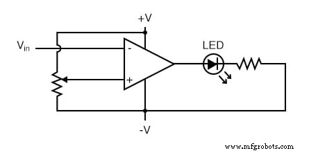
The example circuit compares an input voltage to a reference set by a potentiometer (R₁). If V_in falls below the reference, the output drives an LED; otherwise, the LED stays off. This basic low‑alarm logic can also drive relays, transistors, or SCRs to actuate mechanical devices.

Square‑Wave Converter

Replacing the DC reference with an AC sine wave turns the comparator into a square‑wave generator. Whenever the sine wave crosses the reference, the output toggles between saturation states, producing a square wave whose duty cycle is adjustable via the reference voltage.

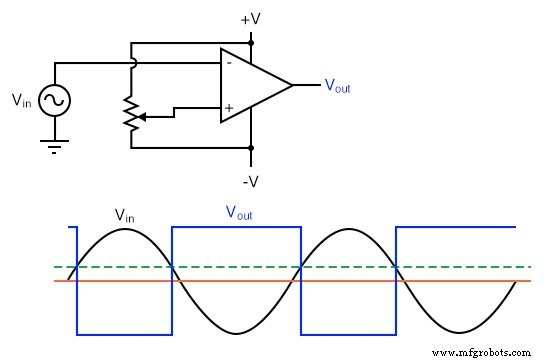
Adjusting the potentiometer changes the crossing point, thereby altering the on/off durations (duty cycle). This principle underlies pulse‑width modulation (PWM), where the pulse width is modulated by a control signal.

Bargraph Driver

Multiple comparator op‑amps, each with a distinct reference voltage but monitoring the same input, can drive a series of LEDs to form a bar graph meter. As the input voltage rises, successive comparators turn on, illuminating more LEDs and visually indicating signal strength.

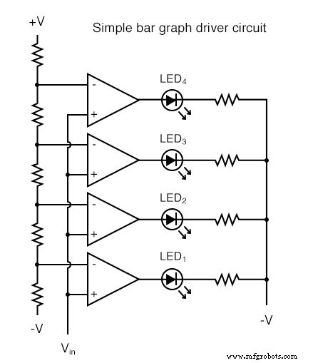
This same architecture is employed in flash analog‑to‑digital converters, where a set of comparators directly translates an analog voltage into a binary code.

Review Summary

• A triangle symbol universally denotes an amplifier circuit.
• All voltages are referenced to a common ground, ensuring consistent measurement.
• A differential amplifier amplifies the voltage difference between two inputs, with (+) as non‑inverting and (–) as inverting.
• An op‑amp is a differential amplifier with ultra‑high gain, originally used in analog computers.
• Op‑amps offer very high input impedance and low output impedance.
• Used as comparators, op‑amps perform rapid “greater‑than” checks, useful for alarms and control logic.
• PWM can be implemented by comparing an AC signal to a DC reference, producing a duty‑cycle‑controlled square wave.

Related Worksheet

• Basic Operational Amplifiers Worksheet