Cascode Amplifier: Combining Common‑Emitter and Common‑Base for Wide Bandwidth and High Input Impedance

While the common‑base (C‑B) amplifier offers a broader bandwidth than the common‑emitter (C‑E) stage, its input impedance—tens of ohms—restricts its usefulness. A common solution is to precede the C‑B stage with a low‑gain C‑E driver that presents a higher input impedance in the kilo‑ohm range.

The stages are arranged in a cascode configuration, stacked in series rather than cascaded as in a conventional amplifier chain.

In a typical capacitor‑coupled, three‑stage common‑emitter amplifier, the cascode topology is employed. It delivers both wide bandwidth and a moderately high input impedance.

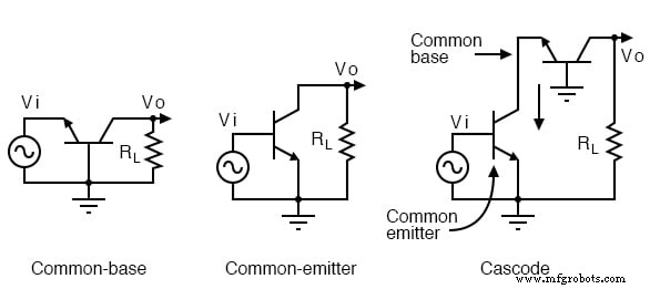
A cascode amplifier combines a common‑emitter stage with a common‑base stage. In AC analysis, power supplies and DC coupling capacitors are modeled as short circuits.

Bandwidth, Capacitance, and the Miller Effect

The cascode’s extended bandwidth stems from the Miller effect. In a C‑E stage, the collector‑base capacitance (Ccbo) is multiplied by the magnitude of the voltage gain (Av). Although Ccbo is smaller than the emitter‑base capacitance, the collector node is 180° out of phase with the base input. The feedback across Ccbo appears as (1 + |Av|) times the physical capacitance, limiting the high‑frequency response of a standalone C‑E amplifier.

The approximate voltage gain of the C‑E amplifier in the figure below is Av = –RL/rEE. With an emitter current of 1.0 mA, the emitter resistance is REE = 26 mΩ/IE = 26 Ω. Thus, Av = –RL/REE = –4700/26 ≈ –181. The pn2222 datasheet lists Ccbo = 8 pF.[FAR] The Miller capacitance is therefore Cmiller = Ccbo(1–Av) = 8 pF × (1–(–181)) ≈ 1456 pF.

A common‑base configuration is not affected by the Miller effect because the grounded base isolates the collector from feeding back to the emitter input. Consequently, a C‑B amplifier exhibits superior high‑frequency performance. To achieve a moderately high input impedance while retaining the benefits of a C‑E stage, the C‑E stage is biased for a low voltage gain of about 1. This reduces the Miller multiplication to 2 × Ccbo.

The key to reducing the C‑E gain is to lower the load resistance. The voltage gain of a C‑E amplifier is approximately RC/RE. With the internal emitter resistance rEE ≈ 26 Ω at 1 mA, and a collector load RC equal to the emitter of the C‑B stage (26 Ω), the gain becomes Av = RC/RE ≈ 1. The Miller capacitance then reduces to Cmiller = Ccbo(1–Av) = 8 pF × (1–(–1)) = 16 pF. We now have a C‑E stage with a moderate input impedance, negligible Miller effect, and no significant voltage gain. The subsequent C‑B stage supplies the high voltage gain (Av ≈ –181). The overall current gain of the cascode equals the β of the C‑E stage, giving a robust overall β.

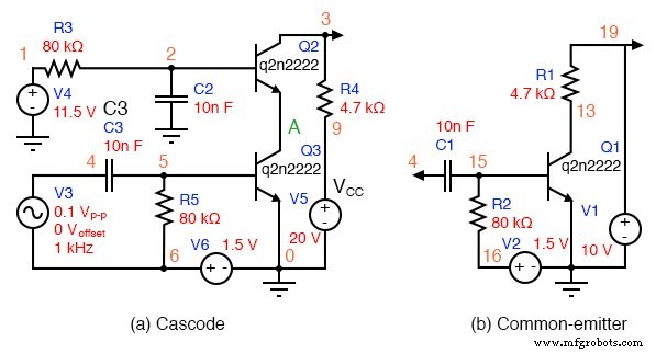
SPICE: Cascode versus Common‑Emitter amplifier comparison.

Cascode vs. Common‑Emitter Amplifier Comparison

The SPICE simulation below compares a cascode amplifier with a standard common‑emitter amplifier. The AC source V3 drives both stages via node 4. Bias resistors are calculated as in the example problem.

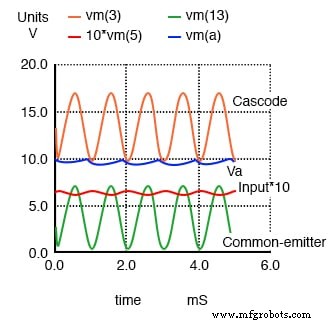
SPICE waveforms. Note that the input is multiplied by 10 for visibility.

SPICE netlist for printing AC input and output voltages.

*SPICE circuit <03502.eps> from XCircuit v3.20 V1 19 0 10 Q1 13 15 0 q2n2222 R1 19 13 4.7k V2 16 0 1.5 C1 4 15 10n R2 15 16 80k Q3 A 5 0 q2n2222 V3 4 6 SIN(0 0.1 1k) ac 1 R3 1 2 80k R4 3 9 4.7k C2 2 0 10n C3 4 5 10n R5 5 6 80k V4 1 0 11.5 V5 9 0 20 V6 6 0 1.5 .model q2n2222 npn (is=19f bf=150 + vaf=100 ikf=0.18 ise=50p ne=2.5 br=7.5 + var=6.4 ikr=12m isc=8.7p nc=1.2 rb=50 + re=0.4 rc=0.3 cje=26p tf=0.5n + cjc=11p tr=7n xtb=1.5 kf=0.032f af=1) .tran 1u 5m .AC DEC 10 1k 100Meg .end

The waveforms illustrate the cascode’s behavior. The input signal is shown amplified tenfold for clarity. Both the cascode and common‑emitter outputs are inverted relative to the input, and the cascode achieves a slightly higher mid‑band gain. The frequency response plots below depict the –3 dB bandwidth of each amplifier.

Note: This section may contain inaccuracies and requires revision. Please refer to the comments at the bottom of the page for more details.

Figure below shows the frequency response of both amplifiers. The SPICE commands responsible for the AC analysis are extracted from the listing:

V3 4 6 SIN(0 0.1 1k) ac 1 .AC DEC 10 1k 100Meg

The cascode demonstrates a marginally better mid‑band gain. For the –3 dB points, the cascode reaches approximately 5 MHz, while the common‑emitter stage tops out near 2 MHz. Thus, the cascode offers a wider bandwidth. The low‑frequency roll‑off is dominated by coupling capacitors and can be mitigated by using larger values. For RF applications, a pair of low‑interelectrode‑capacitance transistors is recommended to achieve even higher bandwidth. Historically, BJT cascode amplifiers were employed in UHF TV tuners before the advent of dual‑gate MOSFETs.

Review

• A cascode amplifier consists of a common‑emitter stage loaded by the emitter of a common‑base stage.
• The heavily loaded C‑E stage has a low gain (~1), which mitigates the Miller effect.
• A cascode amplifier delivers high voltage gain, moderate input impedance, high output impedance, and a wide bandwidth.

Related Worksheets

• Class A BJT Amplifiers Worksheet