Permeability, Saturation, and Magnetic Hysteresis: Interpreting B‑H Curves

To visualize how a material’s permeability varies, we plot the magnetic field intensity (H) on the horizontal axis and the resulting flux density (B) on the vertical axis. Using H (mmf divided by material length) and B (total flux divided by cross‑sectional area) removes dependence on the specimen’s size, enabling a universal comparison of any material’s magnetic response—much like using ohm‑cmil/ft to describe resistance regardless of wire length.

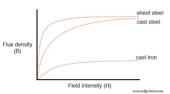
This graph, known as the normal magnetization curve or B‑H curve, reveals the saturation phenomenon. For materials such as cast iron, cast steel, and sheet steel, the flux density flattens as field intensity increases. Initially, only a few magnetic domains align, so additional field force readily increases B. Once the domains are largely aligned, adding more field force yields diminishing returns; the material reaches magnetic saturation and cannot accommodate additional flux.

Air‑core electromagnets never saturate, yet they generate far less flux than a ferromagnetic core for the same number of turns and current.

Magnetic Hysteresis

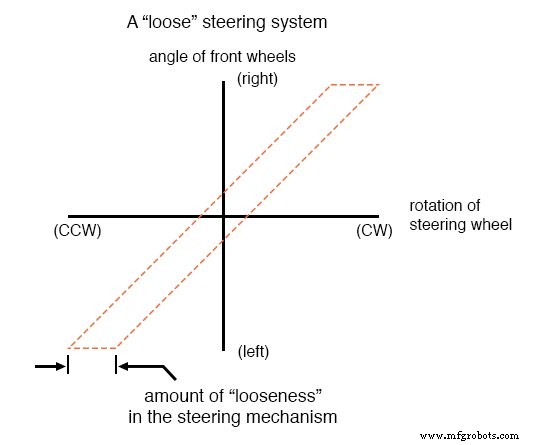
Hysteresis is the lag between an applied magnetic field and the resulting flux. In mechanical systems, steering hysteresis illustrates this: turning a steering wheel left and right requires extra rotation to overcome the linkage’s inherent lag. In magnetic systems, a ferromagnetic core retains magnetization after the applied field is removed—a property known as retentivity. When the field polarity reverses, the core resists demagnetization, producing a characteristic S‑shaped hysteresis loop.

Consider the following sequence:

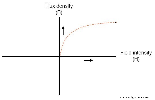
1. Apply a steadily increasing field; B rises along the forward magnetization curve.

2. Cease current; the core retains a residual flux equal to the peak B at zero applied field.

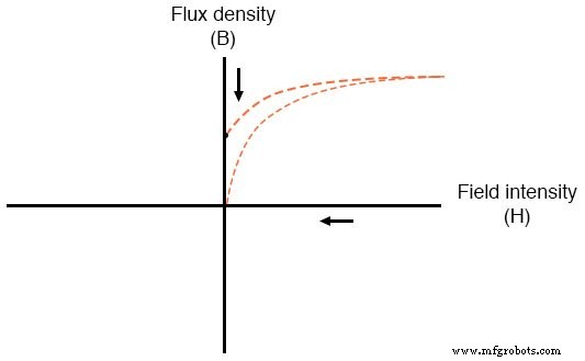
3. Apply reverse field; the flux density follows the reverse branch of the curve until it mirrors the positive peak in the opposite direction.

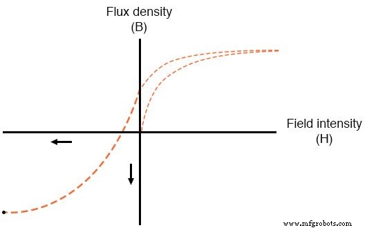
4. Stop current again; the core now holds a residual flux in the negative direction.

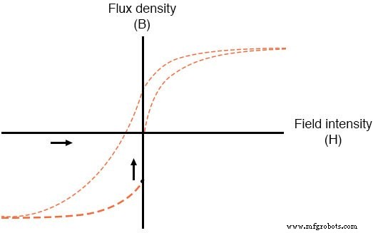
5. Re‑apply positive current; the flux climbs back to the original positive peak, completing the hysteresis loop.

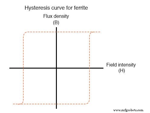
The area enclosed by this loop estimates energy lost to magnetic friction during each cycle.

Example of Hysteresis in Automobiles

Hysteresis also appears in vehicle steering systems. A tight system exhibits a steep curve—steering changes quickly—while a loose system shows a more gradual slope, indicating greater lag.

In precision applications such as racing or electromagnetic circuit design, hysteresis can undermine accuracy or waste energy. Conversely, magnetic storage devices and ferrite noise filters rely on intentional hysteresis to preserve data and attenuate high‑frequency spikes.

Review

• Material permeability varies with the amount of magnetic flux applied.
• The relationship between field intensity (H) and flux density (B) is captured by the normal magnetization (B‑H) curve.
• Excessive field force can push a ferromagnetic material into saturation, beyond which additional flux cannot be accommodated.
• Retentivity leads to hysteresis, a lag in magnetization when the field direction reverses.

Related Worksheets

• Intermediate Electromagnetism and Electromagnetic Induction Worksheet
• Magnetic Units of Measurement Worksheet