Mesh Analysis Explained: Procedure, Examples, and Applications

In electronics, accurately analyzing circuits—especially complex ones with multiple voltage and current sources—requires more than just Kirchhoff’s laws. Mesh (loop) analysis and its extension, supermesh analysis, provide a systematic way to determine currents and voltages using the fewest equations possible.

What Is Mesh Analysis?

Mesh analysis focuses on independent loops (meshes) that contain no other loops inside them. By assigning a mesh current to each loop, we can write Kirchhoff’s voltage law (KVL) for every mesh and solve for the unknown currents. Once the mesh currents are known, branch currents and voltages follow directly via Ohm’s law.

Key Concepts

• Mesh current: A fictitious current that flows around a single mesh, either clockwise or counter‑clockwise.
• Loops containing only one element make the mesh current equal to that element’s current.
• When two meshes share a branch, the branch current equals the algebraic sum (or difference) of the two mesh currents, depending on their directions.

Step‑by‑Step Procedure

1. Identify meshes and assign a mesh current to each, choosing a consistent direction (usually clockwise).
2. Determine the current through every element in terms of the mesh currents.
3. Apply KVL around each mesh to write one equation per mesh, combining voltage drops (V = I·R) and any source voltages.
4. Solve the resulting linear system for the mesh currents.
5. Use the mesh currents to compute branch currents and element voltages.

Setting Up Mesh Equations

Each mesh equation represents the sum of voltage drops around that loop, set equal to zero:

∑V_drop = 0

For a resistor R in a mesh carrying current I, the drop is I·R. If a voltage source V_s lies inside the mesh, its sign depends on the assumed mesh direction: add if you traverse from negative to positive, subtract otherwise.

Illustrative Example

Consider the two‑mesh circuit shown below. Mesh currents I1 and I2 flow clockwise.

Applying KVL yields:

R2(I1 – I2) + R1·I1 = V1  
R2(I2 – I1) + R1·I2 = –V2

Rearranging gives:

I1(R1 + R2) – I2·R2 = V1
–I1·R2 + I2(R1 + R2) = –V2

Solving these equations provides I1 and I2; thereafter, any branch current and voltage can be computed.

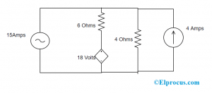
Solving a Three‑Mesh Circuit

The following circuit involves three meshes and several resistors:

Mesh equations:

V1 – R2(I1 – I3) – R4(I1 – I2) = 0
–Vc – R4(I2 – I1) – R3(I2 – I3) = 0
–R1(I3) – R3(I3 – I2) – R2(I3 – I1) = 0

With I2 = –2 A (from the circuit), solving the first and third equations yields I1 ≈ 4.46 A and I3 ≈ –0.615 A. Consequently, Vc ≈ 28.61 V and the branch current I_ac = I1 – I3 ≈ 5.075 A.

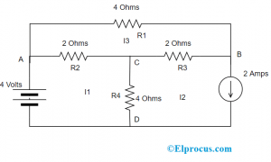
Supermesh Analysis

When a current source lies between two meshes, the two meshes merge into a single supermesh, eliminating the current source from the equations. The supermesh equation is obtained by applying KVL around the combined loop, and an additional constraint equation relates the mesh currents to the source value.

Example: For the circuit below, the supermesh equations are:

10i1 + 80(i1 – i2) + 30(i1 – i3) = 80
30 = 40i3 + 30(i3 – i1) + 20(i2 – i1)
15i_x = i3 – i2

Solving gives i1 ≈ 0.58 A, i2 ≈ –6.16 A, i3 ≈ 2.6 A, and V3 = i3·R3 ≈ 104 V.

Why Use Mesh Analysis?

• Efficient for planar circuits with many elements.
• Reduces the number of unknowns compared to nodal analysis.
• Ideal for circuits containing voltage sources and resistors.
• Facilitates the analysis of unbalanced Wheatstone bridges and other complex topologies.

Mastering mesh and supermesh analysis equips engineers to solve even the most intricate circuits with confidence and precision.