Mastering Mesh Current Analysis: A Comprehensive Guide

The Mesh-Current Method, also called the Loop-Current Method, is a cornerstone of circuit analysis. It uses Kirchhoff’s Voltage Law (KVL) and Ohm’s Law to solve for unknown currents with fewer variables than the Branch-Current method, making hand calculations simpler and faster.

Mesh Current, Conventional Method

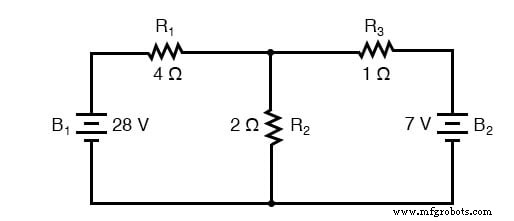
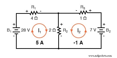
Below is the example circuit we will analyze:

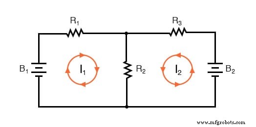
Identify Loops

Step one: mark all independent loops that enclose every component. In this example, loop 1 includes B1, R1, and R2; loop 2 includes B2, R2, and R3. Assign arbitrary directions to the mesh currents (I1, I2). Choosing the same direction for currents that share a resistor—e.g., both I1 and I2 flowing “up” through R2—simplifies the algebra.

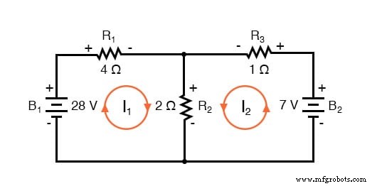
Label Voltage Drop Polarities

Next, mark the polarity of each resistor’s voltage drop relative to the assumed mesh currents. The upstream side of a resistor is negative, the downstream side positive. Battery polarities follow their symbols; they may align or oppose the assumed current direction.

Tracing the Left Loop with KVL

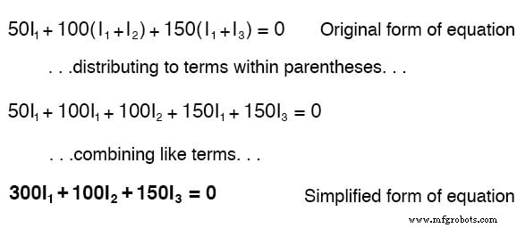
Walking counter‑clockwise around loop 1 and applying KVL yields:

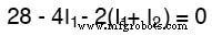
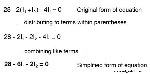
Because R2 carries the sum of I1 and I2, the middle term is 2(I1+I2). Simplifying gives:

Tracing the Right Loop with KVL

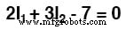
Applying the same procedure to loop 2 gives:

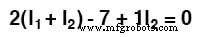
Simplifying:

Solving for the Unknowns

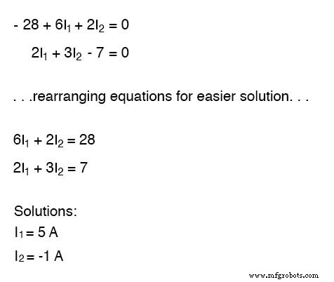
With two linear equations we can solve for I1 and I2 using any standard method (substitution, elimination, matrix inversion). One convenient form is:

Interpreting the Results

Re‑draw the circuit with the solved mesh currents to determine branch currents. A negative I2 indicates the assumed direction was opposite to reality; thus the actual current flows counter‑clockwise at 1 A.

Re‑labeling gives the following branch currents:

• R1: 5 A, voltage drop 20 V (positive left, negative right)
• R3: 1 A, voltage drop 1 V
• R2: I1 down (5 A) and I2 up (1 A) → net 4 A down; voltage drop 8 V

Advantages of Mesh Current Analysis

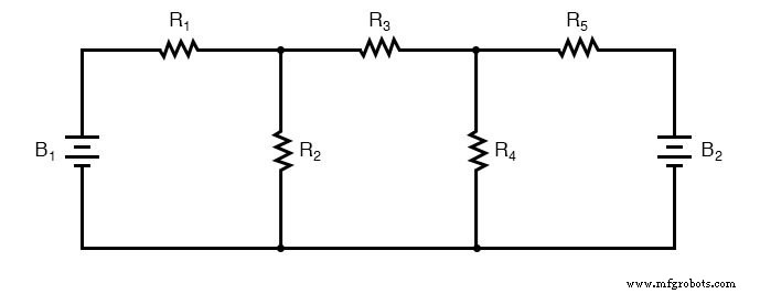
Mesh analysis reduces the number of unknowns and simultaneous equations, especially in larger networks. For the expanded network below, the Branch‑Current method would require five unknowns and five equations, whereas Mesh‑Current needs only three unknowns and three equations.

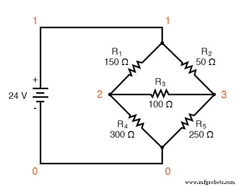
Unbalanced Wheatstone Bridge

Mesh analysis excels in circuits that cannot be reduced by series‑parallel simplification, such as the unbalanced Wheatstone Bridge:

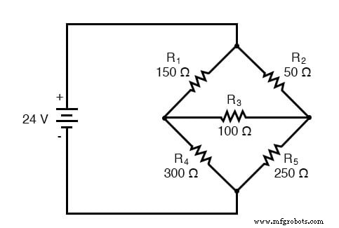
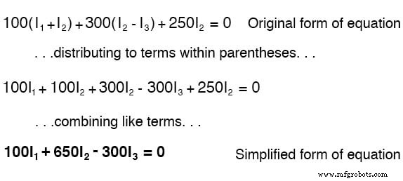
Using Mesh currents, we introduce three loops: I1, I2, and I3 (the latter traverses the battery side). The resulting KVL equations are:

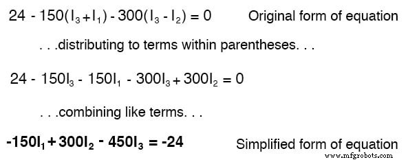
And a third equation to include the source:

Solving the Bridge

Using a matrix solver (e.g., Octave), the currents are:

 octave:1> A = [300,100,150;100,650,-300;-150,300,-450]
 octave:2> b = [0;0;-24]
 octave:3> x = A\b
 x =
  -0.093793
   0.077241
   0.136092

Negative I1 indicates the chosen direction was wrong; the true currents are:

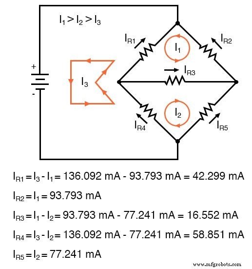
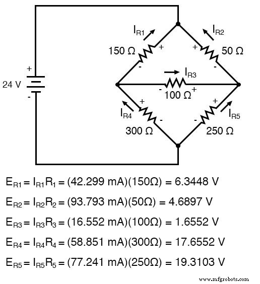
Voltage drops follow from Ohm’s law:

A SPICE simulation confirms the analytical results:

Review of Mesh Current Steps

• Draw enough mesh currents to cover all components.
• Assign arbitrary directions and label resistor polarities.
• Write KVL equations for each loop, replacing each resistor voltage by IR. For shared resistors, use the algebraic sum or difference of mesh currents.
• Solve the simultaneous equations for the mesh currents.
• Any negative solution reveals an incorrect assumed direction.
• Combine mesh currents to find branch currents.
• Compute all voltage drops via E = IR.

Mesh Current by Inspection

When all mesh currents flow clockwise (the conventional direction), the coefficient signs follow a predictable pattern, allowing quick “inspection” equations:

+(sum of loop‑1 resistors)·I1 – (common R1‑2)·I2 – (common R1‑3)·I3 = E1

–(common R1‑2)·I1 + (sum of loop‑2 resistors)·I2 – (common R2‑3)·I3 = E2

–(common R1‑3)·I1 – (common R2‑3)·I2 + (sum of loop‑3 resistors)·I3 = E3

The right‑hand side equals the voltage source seen by the assumed clockwise loop (positive if the loop aligns with the source, negative otherwise). Solving yields the same currents as the systematic method.

For a two‑loop example: loop‑1 resistance 6 Ω, loop‑2 3 Ω, common 2 Ω, with a 28 V source in loop 1 and a 7 V source in loop 2. The resulting currents are I1 = 5 A, I2 = 1 A, both clockwise.

Conclusion

Mesh current analysis is a powerful, efficient technique that reduces complexity, especially in multi‑loop and unbalanced networks. By following the outlined steps, you can reliably solve for currents and voltages with confidence.

Related Worksheet

• DC Mesh Current Analysis Worksheet