Branch Current Method: A Step‑by‑Step Guide to Solving Circuit Networks

The Branch Current Method is the most direct technique for analyzing linear electrical networks. By assigning directions to the currents that flow through each branch and applying Kirchhoff’s Laws, we can formulate a system of simultaneous equations that yields every current and, consequently, every voltage drop in the circuit.

Solving Using Branch Current Method

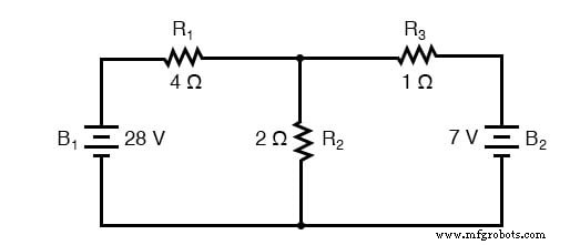
Below is a practical example that walks through the entire process.

Choosing a Node

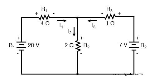
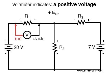
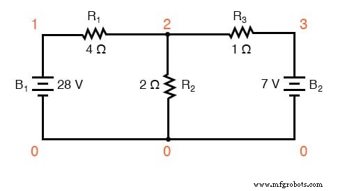
The first step is to select a reference node – the junction where the right side of R₁, the top of R₂, and the left side of R₃ meet. This node will serve as the anchor for all subsequent equations.

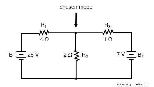
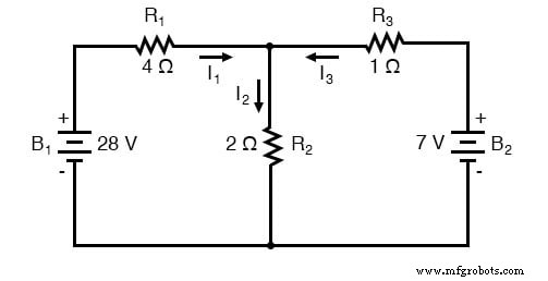
At this node, we tentatively assign directions to the three branch currents, labeling them I₁, I₂, and I₃. These directions are speculative; any incorrect assumption will reveal itself as a negative value in the final solution.

Apply Kirchhoff’s Current Law (KCL)

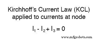
KCL states that the algebraic sum of currents entering and leaving a node must be zero. For our chosen node, we consider currents entering as positive and exiting as negative:

Label All Voltage Drops

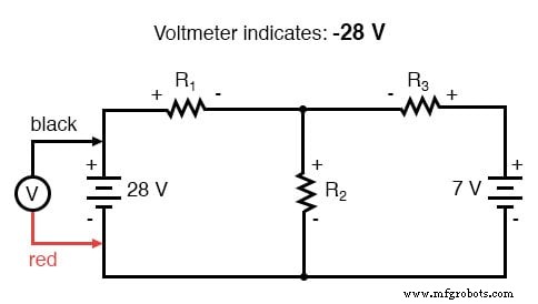
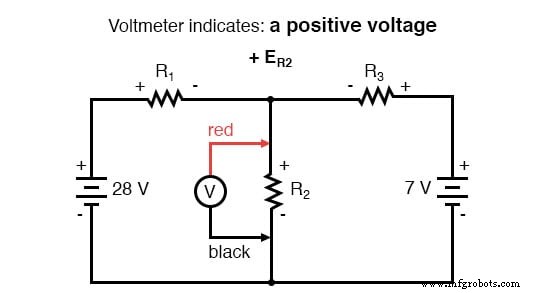
Next, we assign voltage‑drop polarities across each resistor based on the assumed current directions. The positive polarity is where current enters the resistor; the negative polarity is where it exits:

Battery polarities remain as indicated by their symbols (short end negative, long end positive). It is acceptable for a resistor’s voltage polarity to differ from a nearby battery’s polarity—as long as the resistor’s polarity reflects the assumed current direction. Incorrect current assumptions will surface as negative solutions, but the magnitudes will still be correct.

Apply Kirchhoff’s Voltage Law (KVL)

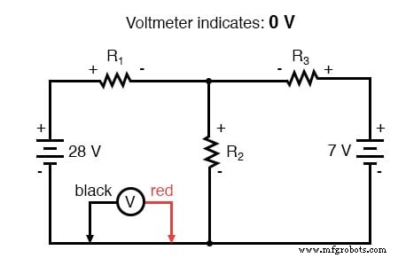
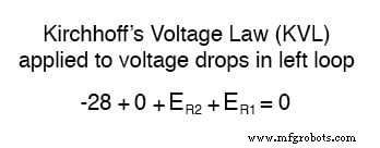
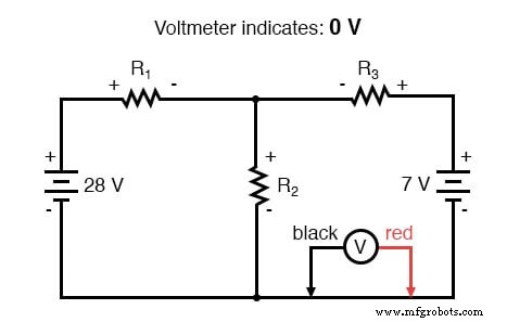
KVL requires that the algebraic sum of all voltage changes around any closed loop be zero. We trace the left loop counter‑clockwise, starting at the upper‑left corner:

Summing the voltage contributions gives the KVL equation for the left loop:

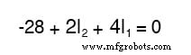
Because the resistor voltages are unknown at this stage, we express them as the product of the corresponding currents and resistances (Ohm’s Law, E = IR). Substituting the known resistor values simplifies the equation:

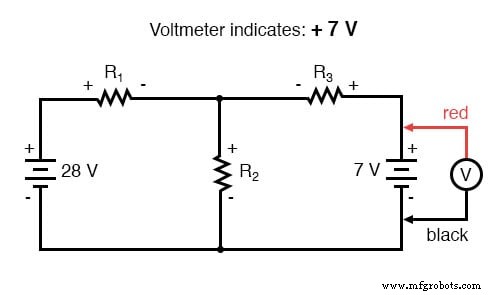
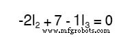
We perform the same procedure for the right loop, obtaining a second KVL equation:

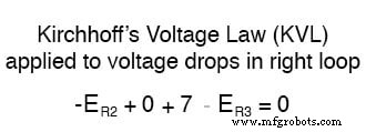
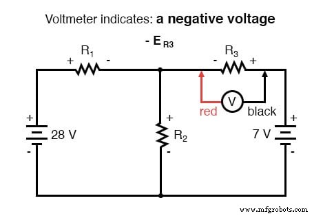
Expressing each resistor voltage as the product of current and resistance yields:

Solving For the Unknown

We now have three equations – one KCL and two KVL – involving the three unknown currents I₁, I₂, and I₃:

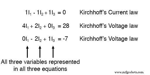
Rearranging the equations to isolate constants on the right side makes solving easier:

Solving this system yields:

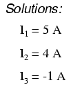
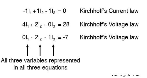
Thus, I₁ = 5 A, I₂ = 4 A, and I₃ = –1 A. The negative value indicates that the actual direction of I₃ is opposite to our initial assumption. We can correct the diagram accordingly:

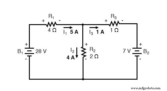
Redraw The Circuit

The updated diagram shows current flowing against the orientation of the second battery because the first battery’s higher voltage forces electrons backward through that branch. This outcome demonstrates that a stronger battery does not always dominate; the relative voltages and resistor values jointly determine the final current directions.

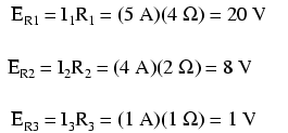
Calculate The Voltage Drop Across All Resistors

With the current magnitudes known, we compute each resistor’s voltage drop using Ohm’s Law:

Analyze Network Using SPICE

To confirm our analytical results, we simulate the circuit in SPICE. The following netlist demonstrates the setup:

network analysis example
 v1 1 0
 v2 3 0 dc 7
 r1 1 2 4
 r2 2 0 2
 r3 2 3 1
 .dc v1 28 28 1
 .print dc v(1,2) v(2,0) v(2,3)
 .end
 v1 v(1,2) v(2) v(2,3)
 2.800E+01 2.000E+01 8.000E+00 1.000E+00

The SPICE output confirms the voltage drops: 20 V across R₁, 8 V across R₂, and 1 V across R₃. All values are positive, indicating that the node numbering matches the polarities derived analytically.

REVIEW:

• Choose a node and assume branch current directions.
• Write a KCL equation for that node.
• Assign resistor voltage‑drop polarities based on the assumed currents.
• Write KVL equations for each independent loop, replacing resistor voltages with IR.
• Solve the resulting system of simultaneous equations for the unknown currents.
• If any current solution is negative, the assumed direction was incorrect; reverse the arrow and recalculate the polarity.
• Compute all resistor voltage drops using E = IR.

RELATED WORKSHEET:

• DC Branch Current Analysis Worksheet