Understanding Q Factor and Bandwidth in Resonant Circuits: Theory, Calculations, and Practical Design

The Q, or quality, factor of a resonant circuit quantifies its selectivity and energy efficiency. A higher Q means a narrower bandwidth, which is crucial for filtering, tuning, and RF design.

Mathematically, Q is the ratio of power stored in the reactive elements to power dissipated in the resistive component:

Q = P_{stored}/P_{dissipated} = I^2X/I^2R = X/R
where:
X = capacitive or inductive reactance at resonance
R = series resistance

This expression holds for series resonators and for parallel resonators when the series resistance of the inductor dominates. In practice, the inductor’s DC resistance limits the attainable Q.

Note: Some texts present the formula with X and R swapped for a parallel resonator with a large parallel resistance. Our formula is correct for the common case of a small series resistance in the inductor.

In a series resonator, the voltage across the inductor or capacitor can reach Q times the total applied voltage. In a parallel resonator, the current through the reactive elements can reach Q times the total applied current.

Series Resonant Circuits

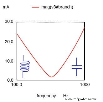
At resonance, a series resonator behaves like a pure resistor: the inductive and capacitive reactances cancel, leaving only the series resistance to determine impedance. This gives the minimum impedance and maximum current.

Below resonance, the circuit appears capacitive because the capacitor’s reactance dominates. Above resonance, it appears inductive as the inductor’s reactance grows.

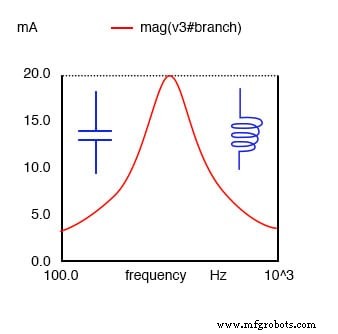
At resonance the series resonant circuit appears purely resistive. Below resonance it looks capacitive; above it appears inductive.

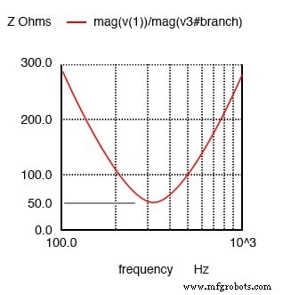
Impedance is at a minimum at resonance in a series resonant circuit.

The peak current can be tuned by adjusting the series resistance, which in turn changes Q and the breadth of the resonance curve. A low‑resistance, high‑Q circuit yields a sharp, narrow peak; a high‑resistance, low‑Q circuit produces a broad, gentle response.

Bandwidth is directly related to Q and the resonant frequency:

BW = f_c / Q

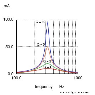
A high‑Q resonant circuit has a narrow bandwidth compared to a low‑Q circuit.

The bandwidth is defined as the frequency range between the 0.707 (≈70.7%) current amplitude points, corresponding to the half‑power points since P = I^2R.

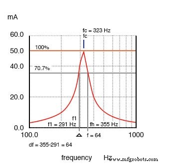
Bandwidth, Δf, is measured between the 70.7% amplitude points of a series resonant circuit.

BW = Δf = f_h - f_l = f_c / Q
where:
  f_h = high‑band edge
  f_l = low‑band edge
  f_c = center (resonant) frequency

In the example above, the 100% current point is 50 mA. The 70.7% level is 35.4 mA. The band edges read 291 Hz (f_l) and 355 Hz (f_h). The bandwidth is 64 Hz, and the half‑power points are ±32 Hz around the center frequency:

BW = Δf = 355 Hz - 291 Hz = 64 Hz
f_l = f_c - Δf/2 = 323 Hz - 32 Hz = 291 Hz
f_h = f_c + Δf/2 = 323 Hz + 32 Hz = 355 Hz
Q = f_c / BW = 323 Hz / 64 Hz ≈ 5

Parallel Resonant Circuits

A parallel resonator reaches its maximum impedance at resonance. Below resonance it behaves inductively because the inductor’s lower impedance draws more current. Above resonance it behaves capacitively as the capacitor’s lower impedance dominates.

A parallel resonant circuit is resistive at resonance, inductive below resonance, and capacitive above resonance.

Because voltage equals impedance times current (V = I·Z), the voltage peaks at resonance where impedance is highest.

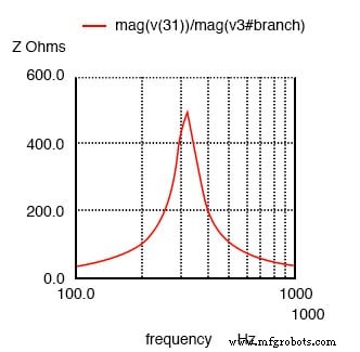
Parallel resonant circuit: Impedance peaks at resonance.

In practice, a low Q—caused by a high series resistance in the inductor—produces a modest, broad peak. A high Q—achieved with a low‑resistance, high‑diameter wire—yields a pronounced, narrow peak. Adjusting the inductor’s winding gauge and wire gauge directly influences Q.

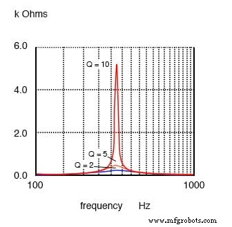
Parallel resonant response varies with Q.

The bandwidth of a parallel resonator is measured between the half‑power voltage points (70.7% impedance points). Since power ∝ V^2, these points represent the 50% power level.

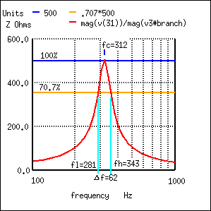
Bandwidth, Δf, is measured between the 70.7% impedance points of a parallel resonant circuit.

In the example, the 100% impedance point is 500 Ω. The 70.7% level is 354 Ω. The band edges read 281 Hz (f_l) and 343 Hz (f_h). The bandwidth is 62 Hz, and the half‑power points are ±31 Hz around the center frequency:

BW = Δf = 343 Hz - 281 Hz = 62 Hz
f_l = f_c - Δf/2 = 312 Hz - 31 Hz = 281 Hz
f_h = f_c + Δf/2 = 312 Hz + 31 Hz = 343 Hz
Q = f_c / BW = 312 Hz / 62 Hz ≈ 5

RELATED WORKSHEETS:

• Resonance Worksheet
• Algebraic Substitution for Electric Circuits Worksheet