Mastering Series RLC Circuit Analysis: From Impedance to KVL

In this article we walk through a practical example of a series RLC circuit and show how to analyze it using complex impedance, Ohm’s law, and Kirchhoff’s voltage law.

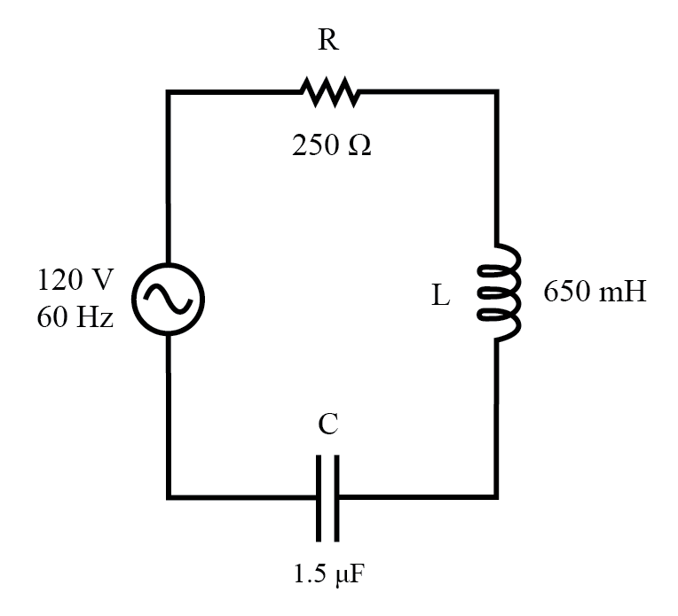
Series R, L, and C circuit.

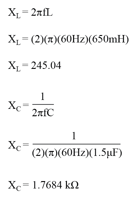
Step 1: Calculate Reactances

First, compute the inductive and capacitive reactances:

Step 2: Convert to Impedance

Express each element as a complex impedance. Remember that an inductor contributes a positive imaginary component (+jX_L), a capacitor a negative imaginary component (–jX_C), and a resistor remains purely real (R).

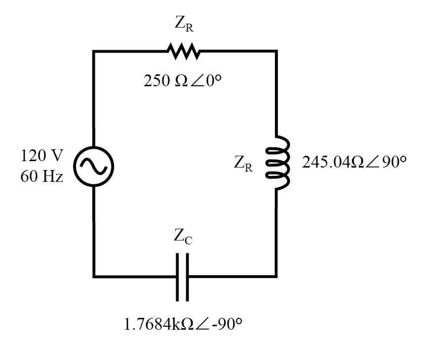
Series RLC circuit with impedances substituted for component values.

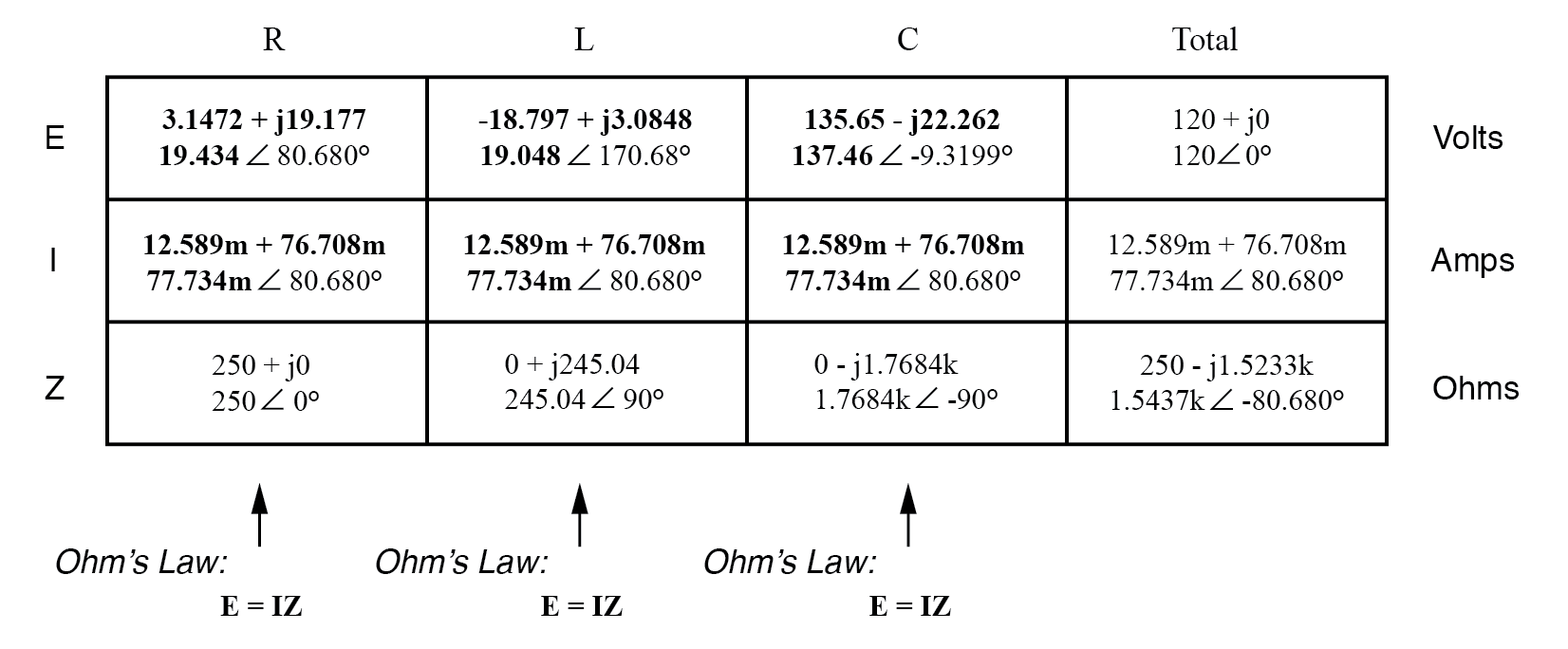
Tabulate the Quantities

With all opposition expressed as complex numbers, the circuit behaves like a DC network where each impedance can be treated as a resistor.

Populate a table with the supplied voltage, component impedances, and any known values:

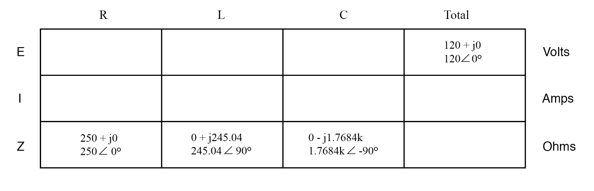
The source voltage is taken as the reference (0°). Phase angles of the individual impedances are absolute: +90° for the inductor, –90° for the capacitor.

For simplicity, we assume ideal reactive components throughout this example.

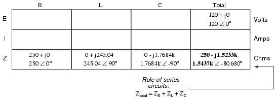
Because the circuit is series, the total impedance is the algebraic sum of the individual impedances:

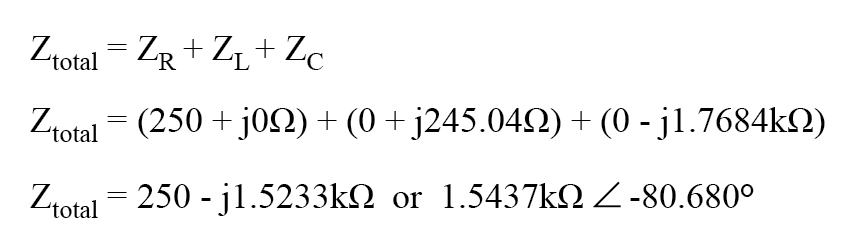
Insert this into the table:

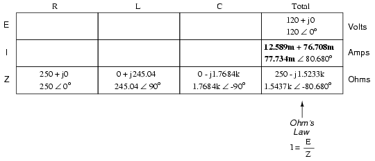
Apply Ohm’s Law

Using I = E/Z, calculate the total current for the series network:

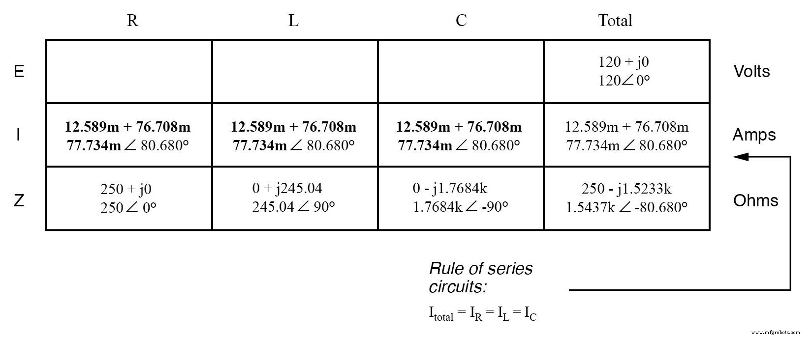
Since the circuit is series, the same current flows through every element. Distribute this current across the table:

Determine Voltage Drops

Apply V = IZ to each component to find the voltage drop across the resistor, inductor, and capacitor:

Notice that the supply voltage is only 120 V, yet the capacitor’s voltage is 137.46 V. This apparent paradox is explained by the cancellation effect between the inductive and capacitive reactances.

In series, the inductive (+jX_L) and capacitive (–jX_C) reactances oppose each other, reducing the total impedance. A lower impedance yields a higher current, which can produce individual voltage drops that exceed the source voltage.

Once all component values are expressed as impedances, AC circuit analysis reduces to DC analysis with the only difference being the handling of vector quantities.

Power calculations remain the unique element that differs between AC and DC analysis.

Verify with Kirchhoff’s Voltage Law

KVL states that the algebraic sum of the voltage drops must equal the source voltage. Complex addition confirms this:

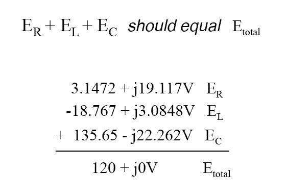
Even though the individual drops look larger than the source, their vector sum is exactly 120 V (120 + j0 V). Rounding errors are negligible when all significant digits are retained.

Simulation Check with SPICE

Below is a SPICE netlist for the same circuit:

r1 1 2 250
l1 2 3 650m
c1 3 0 1.5u
.ac lin 1 60 60
.print ac v(1,2) v(2,3) v(3,0) i(v1)
.print ac vp(1,2) vp(2,3) vp(3,0) ip(v1)
.end

SPICE results confirm the hand‑calculated values:

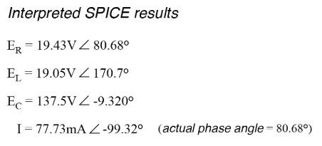
Simulation aligns with analytic calculations.

Key Takeaways

• Series impedances add directly: Z_total = ΣZ_i.
• In a series RLC circuit, inductive and capacitive reactances can cancel, reducing total impedance and potentially increasing individual voltage drops beyond the supply.
• All DC circuit rules apply to AC when quantities are expressed as complex impedances, except for power calculations, which require separate treatment.

Further Practice

• Series‑Parallel Combination AC Circuits Worksheet