Impedance Transformation with Transmission Lines: Matching Techniques Using Standing Waves

At the resonant frequency of a transmission line, standing waves arise that can dramatically alter the impedance perceived by the source. When the line length equals an integer multiple of half a wavelength (λ/2, λ, 3λ/2, …), the source “sees” the termination impedance unchanged.

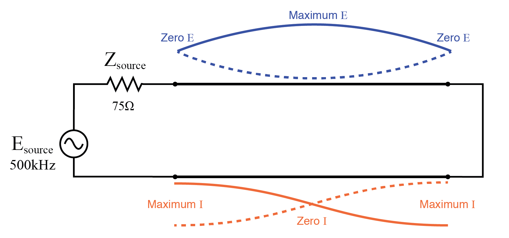
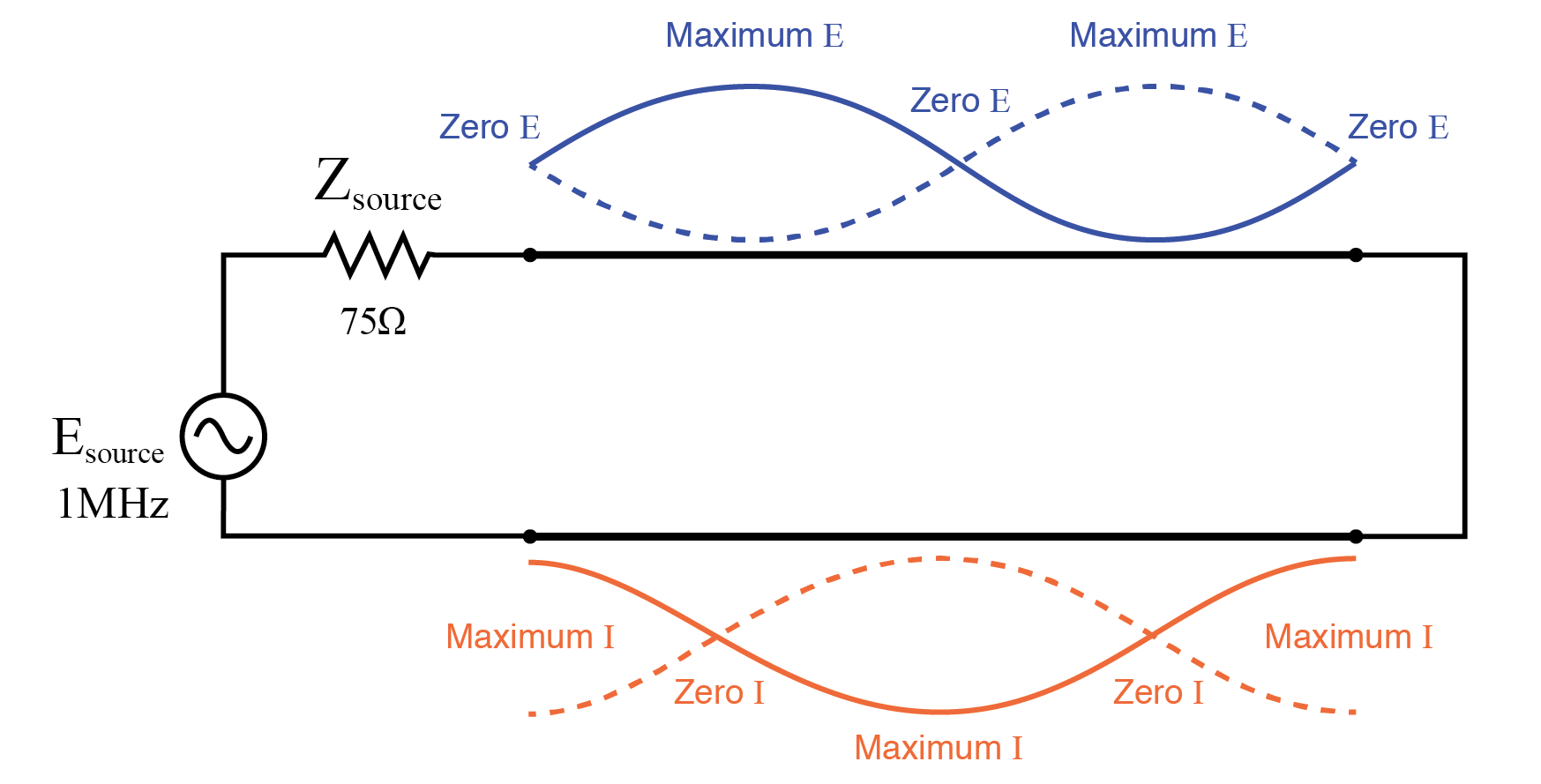
Illustrations below show an open‑circuited line operating at λ/2 and λ frequencies:

 

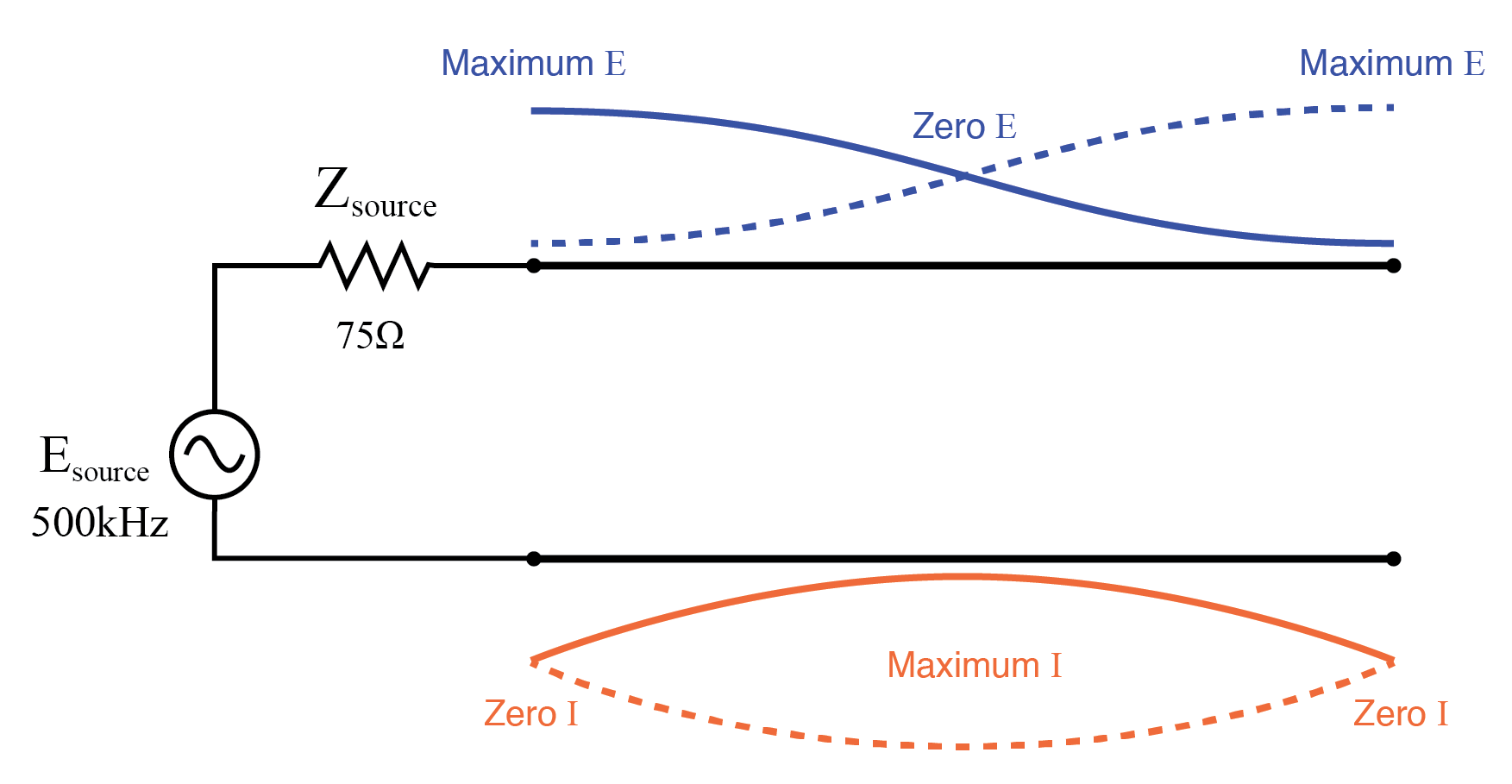
Source sees open, identical to the load at the end of a λ/2 line.

 

Source sees open, identical to the load at the end of a full‑wave (2×λ/2) line.

 

In both cases the line exhibits voltage antinodes and current nodes at its ends – the hallmark of an open circuit. This symmetry ensures that the line faithfully reproduces its terminating impedance at the source end.

The same principle applies to a short‑circuited line. At frequencies where the line length is a half‑wave multiple, the source “sees” a short circuit, with minimum voltage and maximum current at the source–line junction.

 

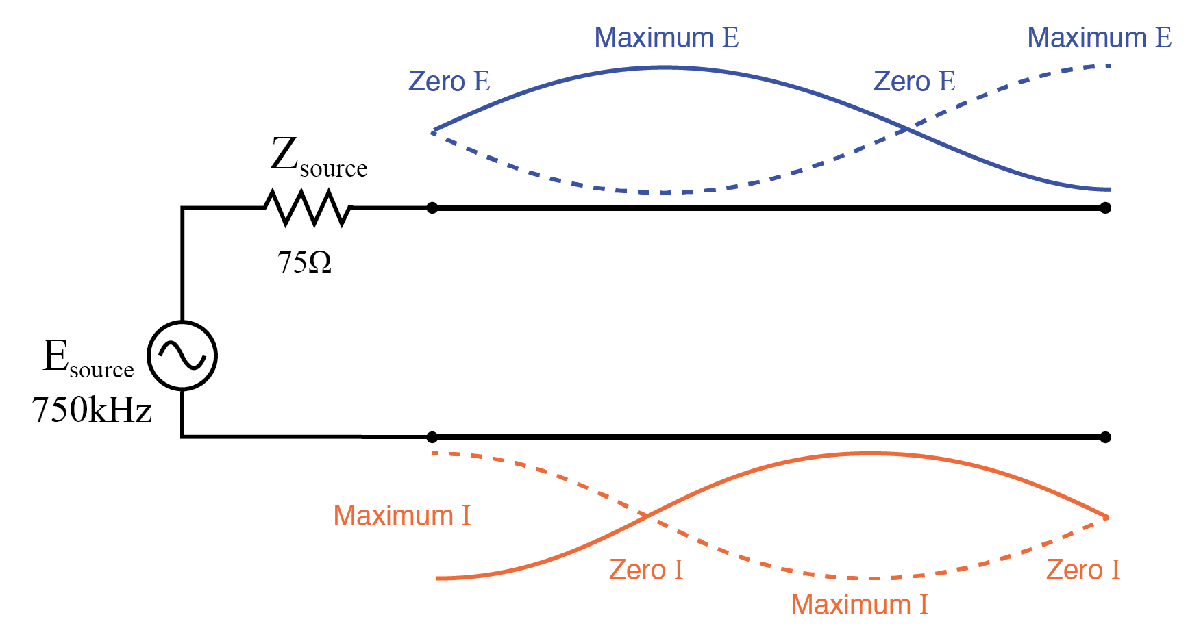
Source sees short, identical to the load at the end of a λ/2 line.

 

Source sees short, identical to the load at the end of a full‑wave line.

 

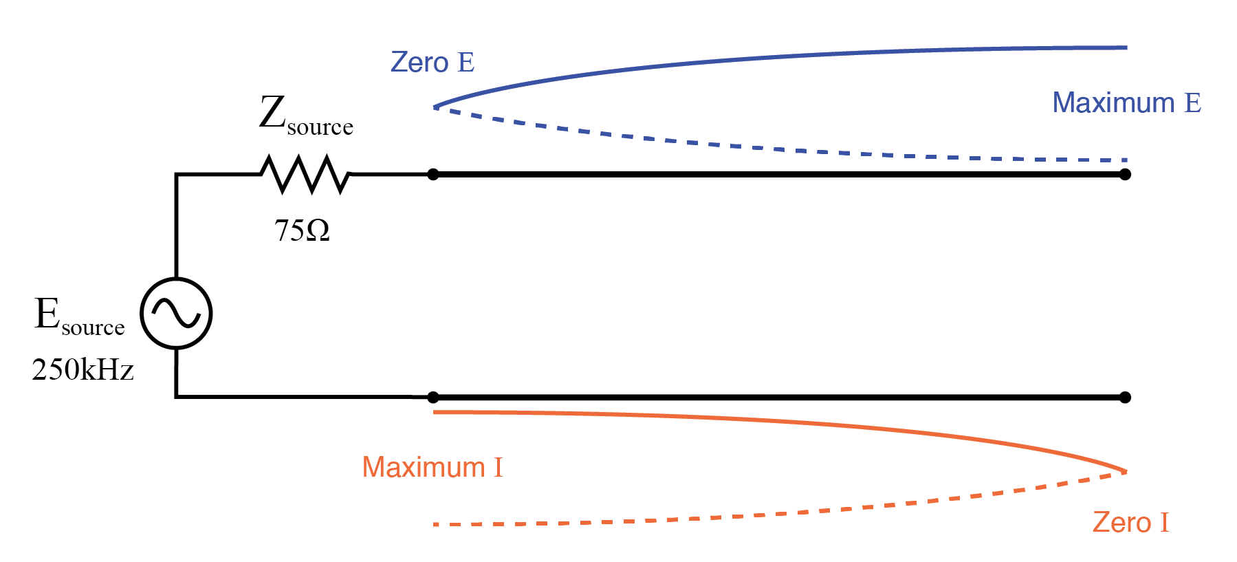
However, when the line resonates at a quarter wavelength (λ/4) or an odd multiple thereof, the source “sees” the opposite impedance of the termination.

For example, an open‑circuited line behaves as a short at its source end when its length equals λ/4 or 3λ/4. Conversely, a short‑circuited line appears as an open at λ/4 or 3λ/4.

Open‑circuited line – source sees short:

 

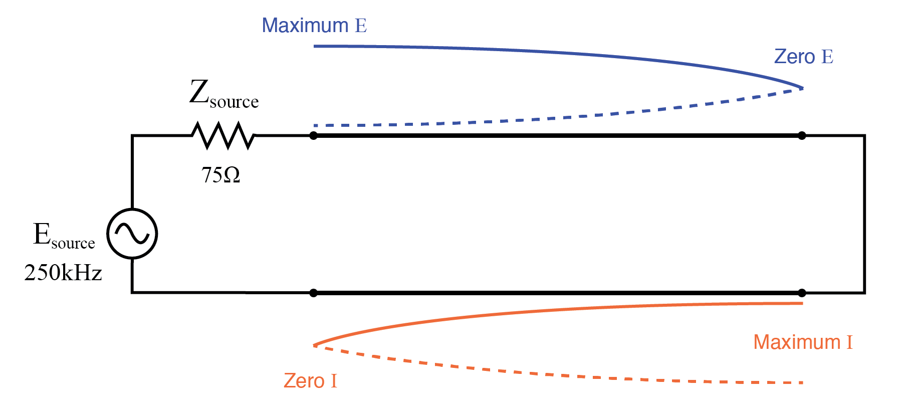
Source sees short, reflected from the open load at λ/4.

 

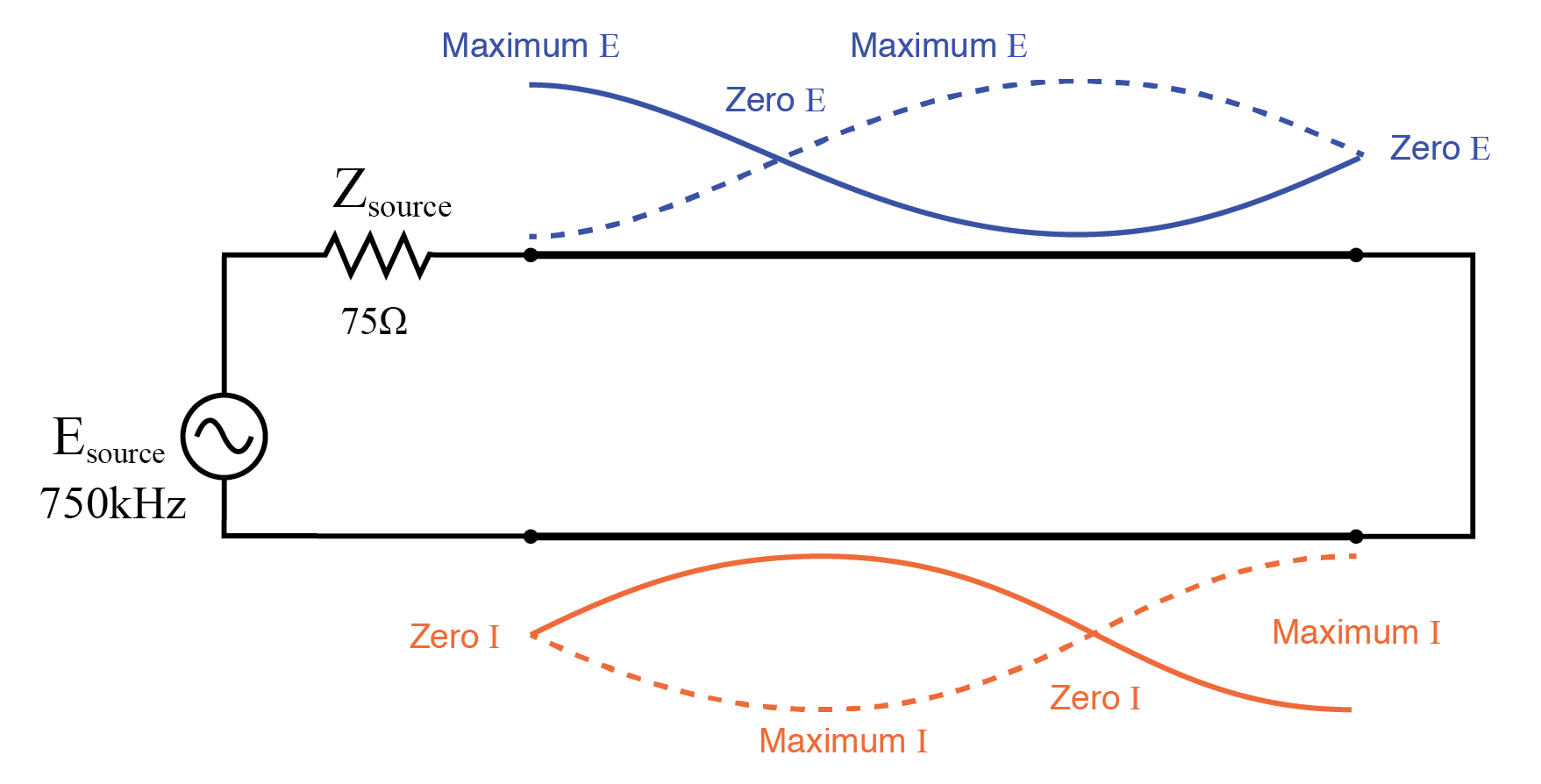
Source sees short, reflected from the open load at 3λ/4.

 

Short‑circuited line – source sees open:

 

Source sees open, reflected from the short load at λ/4.

 

Source sees open, reflected from the short load at 3λ/4.

 

At these resonant points the line functions as an impedance transformer, converting an infinite impedance to zero or vice versa. Although this effect occurs only at specific frequencies, it can be exploited to match otherwise incompatible impedances when the operating frequency is fixed.

Consider a 75 Ω source feeding a 100 Ω load through a 75 Ω transmission line. Using SPICE, the impedance seen by the source at various resonant lengths is:

 

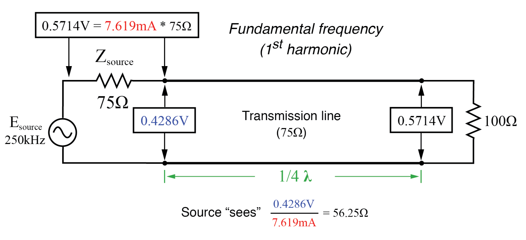
Source sees 56.25 Ω at λ/4.

 

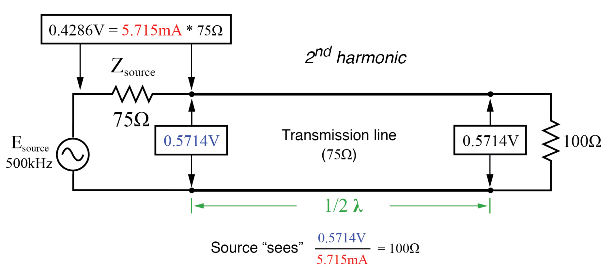
Source sees 100 Ω at λ/2.

 

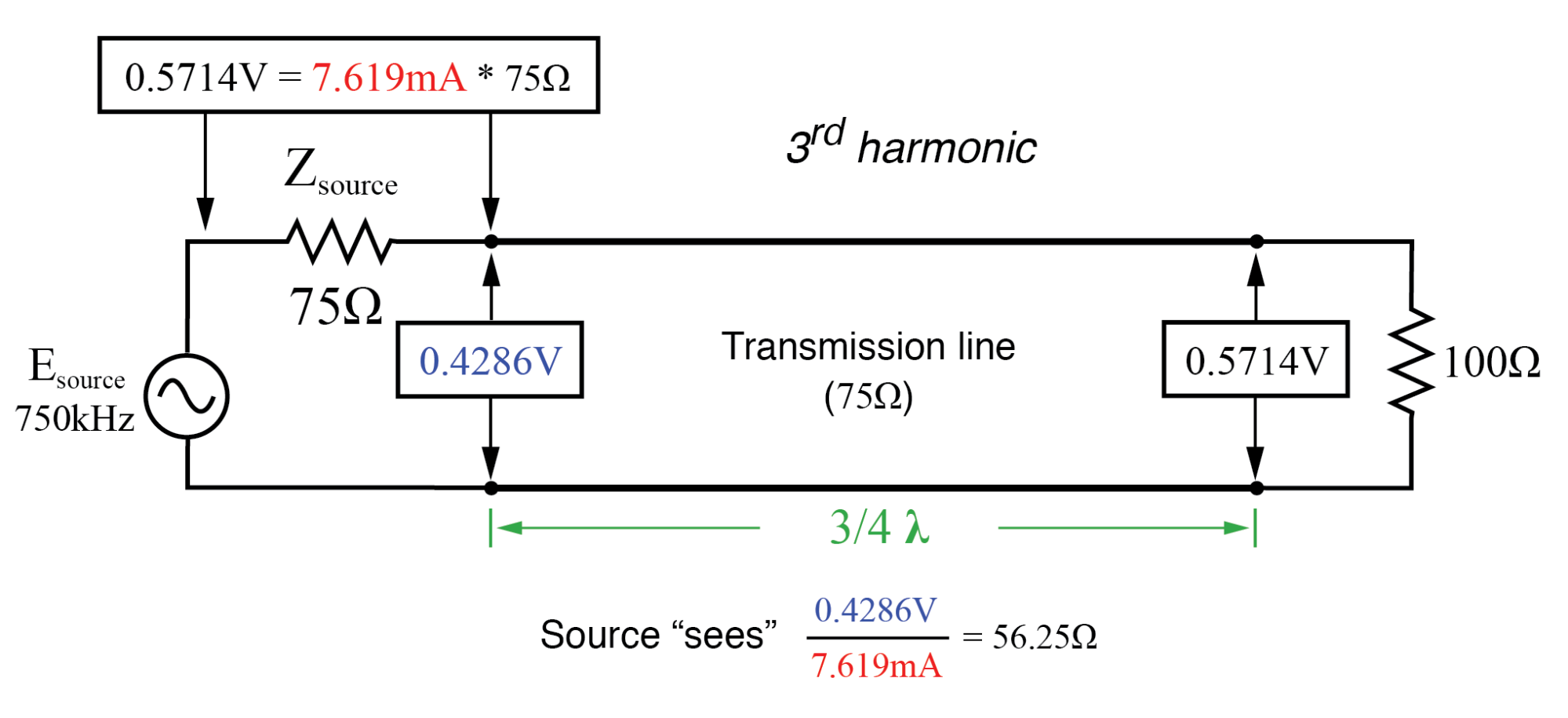
Source sees 56.25 Ω at 3λ/4 (identical to λ/4).

 

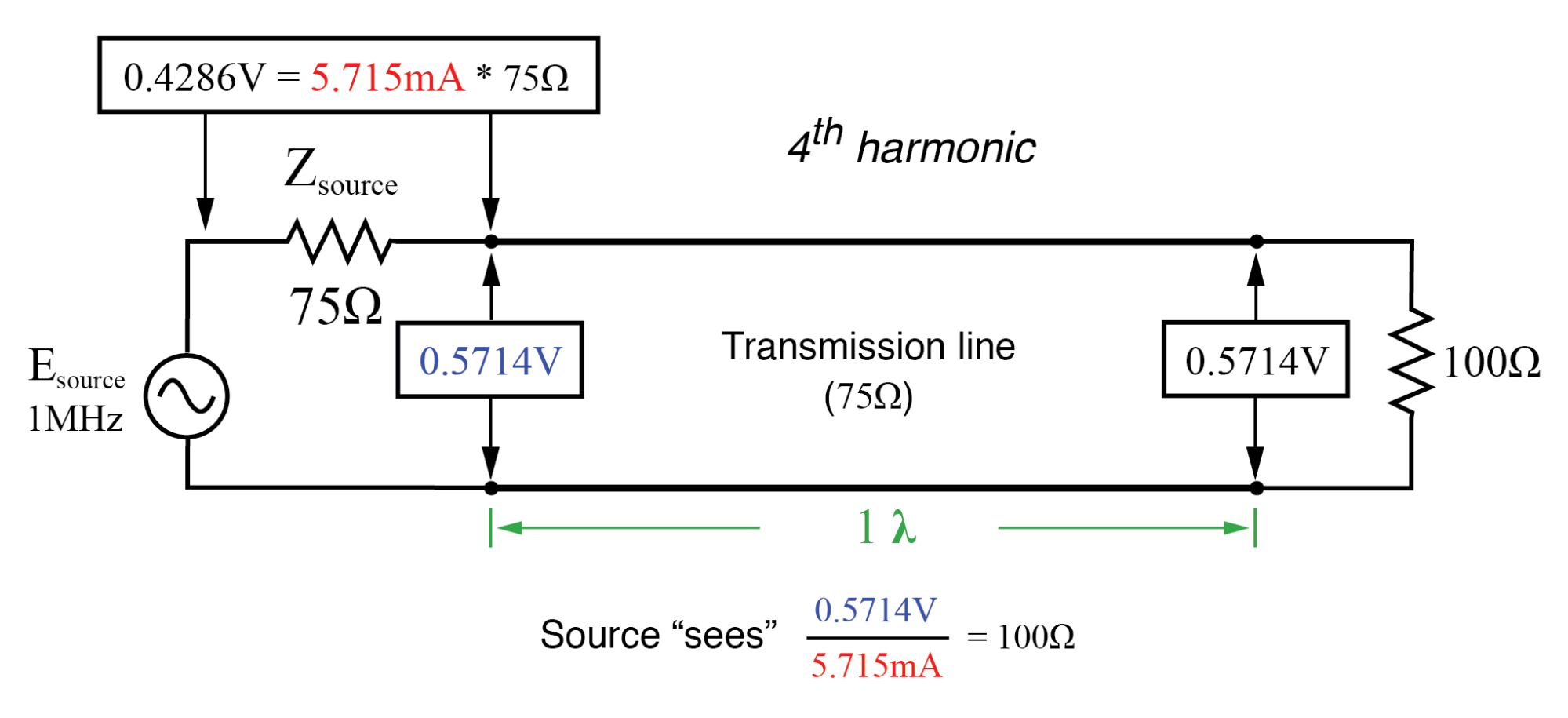
Source sees 100 Ω at full wavelength (identical to λ/2).

 

Relationship Between Line, Load, and Input Impedance

For an unmatched line operating at an odd harmonic of its fundamental, the input impedance is given by:

 

 

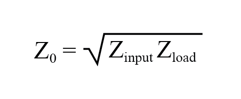
This simple expression is the foundation of many practical matching networks.

Example: Matching a 300 Ω load to a 75 Ω source at 50 MHz. First compute the required characteristic impedance:

Z₀ = √(Z_S × Z_L) = √(75 × 300) = 150 Ω.

With a velocity factor of 0.85 (v ≈ 158 100 mi/s) the 50 MHz wavelength is 16.695 ft. A quarter‑wave section is therefore 4.174 ft long.

The SPICE model is:

Transmission line
v1 1 0 ac 1 sin
rsource 1 2 75
t1 2 0 3 0 z0=150 td=5n
rload 3 0 300
.ac lin 1 50meg 50meg
.print ac v(1,2) v(1) v(2) v(3)
.end

Simulation results at 50 MHz:

freq          v(1,2)      v(1)        v(2)        v(3)
5.000E+07     5.000E-01   1.000E+00   5.000E-01   1.000E+00

The source voltage splits evenly between its 75 Ω internal resistance and the line’s input, making the load appear as 75 Ω to the source. The full 1 V appears at the 300 Ω load, delivering the maximum power transfer predicted by the theorem.

Because this matching is frequency‑specific, the quarter‑wave line must be tuned for each operating frequency. The same 150 Ω line can also match a 75 Ω load to a 300 Ω source, illustrating the reciprocity of impedance transformation.

Impedance matching with a quarter‑wave transformer is a standard technique in RF transmitters, where the carrier frequency is known and stable. The brevity of a λ/4 section offers the shortest possible conductor length.

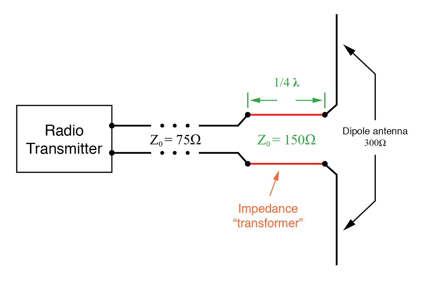
150 Ω quarter‑wave line matches a 75 Ω transmission line to a 300 Ω antenna.

 

Key Takeaways

• A transmission line with standing waves can match disparate impedances when operated at the correct frequency.
• At a λ/4 standing wave, the required characteristic impedance is √(Z_S × Z_L).