Compensation Theorem in Circuit Analysis: Proof, Explanation, and Practical Examples

Proof, Explanation, Experiment and Solved Examples of Compensation Theorem for Circuit Analysis

Compensation Theorem

Sime times in network theory, it is important to know or study the effect of change in impedance in one of its branches. It will affect the corresponding voltage and currents of the network or circuit. The compensation theorem gives information about the change in the network.

The compensation theorem works on the basic concept of Ohm’s law. According to Ohm’s law, when a current passes through the resistor, some amount of voltage drop occurs across the resistor. This voltage drop will oppose the source voltage.

Therefore, we connect an extra voltage source in opposite polarity compared to the source voltage and magnitude is equal to the voltage drop. The compensation theorem works on this concept.

Compensation theorem states that,

• Related Post: Thevenin’s Theorem. Step by Step Guide with Solved Example

Explanation of Compensation Theorem

To understand the compensation theorem, consider the below figure.

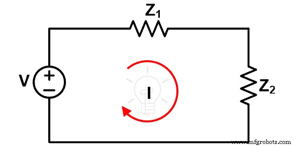
In this figure, the voltage source V is an independent voltage and source and two impedances Z₁ and Z₂ are linear or bilateral elements. Therefore, we can apply the compensation theorem to this network. The current that passes through the loop is I.

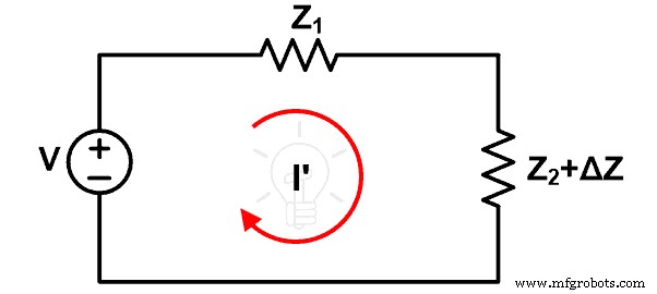
Now, assume that the impedance Z₂ increased by ∆Z. Due to this change, the current passes through the loop is changed and it is I’. The new circuit diagram is shown in the figure below.

Due to the change in impedance, the change in current given by ∆I.

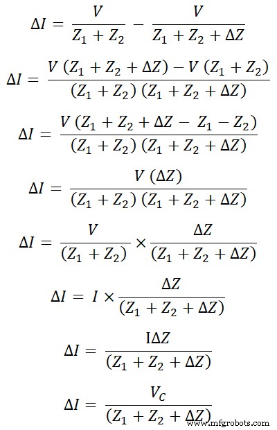
ΔI = I – I’

According to the statement of compensation theorem, we can directly calculate the change in the current ∆I. For that, we need to modify the circuit.

The first modification is that, connect a voltage source of value I∆Z in the branch of which impedance is changed. And the polarity of this voltage source is opposite to the main source. The newly added voltage source V_C is known as the compensation source.

V_C = I ΔZ

The second modification is that we need to remove the old voltage source by its internal impedance. If we consider an ideal voltage source, in this condition, we can remove this voltage source by short-circuiting its terminal. After these modifications, the remaining circuit is as shown in the figure below.

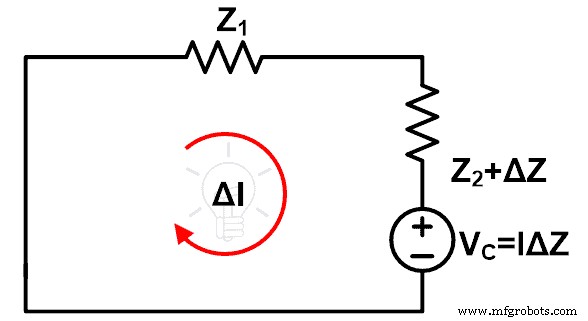
By solving the above circuit, we can easily find the change in current after the change in the impedance.

• Related Post: Norton’s Theorem. Step by Step Guide with Solved Example

Proof of Compensation Theorem

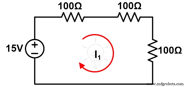
Consider the circuit given in the figure-1. Calculate the current (I) passing through the loop.

Apply KVL to the figure-1;

Now, we have assumed that the impedance Z₂ is changed by ∆Z. And the modified circuit is as shown in figure-2. We need to calculate (I’) the current passes through the loop in figure-2.

Apply KVL to the figure-2;

Due to the change in impedance, the change in loop current is denoted as ∆I. And the ∆I is equal to the difference between old current I and new current I’.

ΔI = I – I’

Now, consider the below figure.

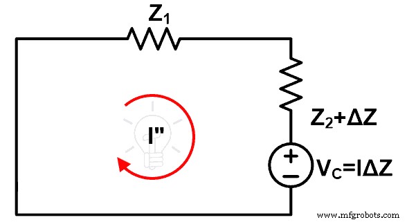
This figure represents the circuit after the implementation of the compensation theorem. Here, the original voltage source is removed by short-circuiting (assume ideal voltage source).

We will find the current passes through this loop that is I”. And compare this current with the current calculated above.

To calculate the current that passes through the loop, apply KVL to the above figure.

V_C = Z₁ I” +(Z₂ +ΔZ) I”

V_C = I” (Z₁ + Z₂ + ΔZ)

I” = V_C / (Z₁ + Z₂ + ΔZ)

I” = ΔI

Hence, it is proved that the change in current (∆I) after modification is the same as the current calculated by the compensation theorem.

And we have proved the statement of compensation theorem.

• Related Post: Superposition Theorem – Circuit Analysis with Solved Example

An Experiment of Compensation Theorem

Aim: Prove the compensation theorem and find the change in current.

Apparatus: Voltmeter, Ammeter, Resistors, Connecting wires, Breadboard,

Circuit diagram:

Procedure:

Step-1 Connect the components as shown in figure-5 using connecting wire on a breadboard.

Step-2 Measure the current I.

Step-3 Connect the components as shown in figure-6. Here, we have connected an extra resistor.

Step-4 Measure the current I1.

Step-5 Calculate the change in current (∆I) from the value of I and I1.

Step-6 Connect the components as shown in figure-7. This circuit is a compensation circuit.

Step-7 Measure the current I”.

Step-8 Compare the change in current (∆I) with the I”.

Experiment Table:

Sr. No.	I	I1	∆I	I”
1

Result:

By comparing the value of current I’’ with ∆I, we can prove the compensation theorem.

• Related Post: Millman’s Theorem – Analyzing AC & DC Circuits – Examples

Example of Compensation Theorem

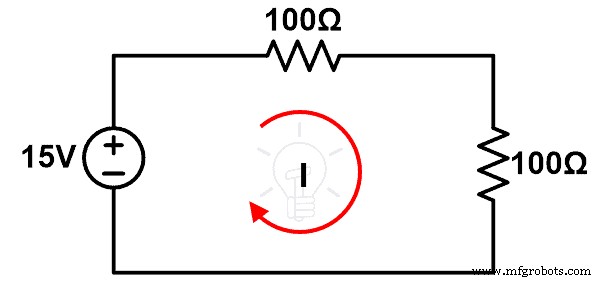
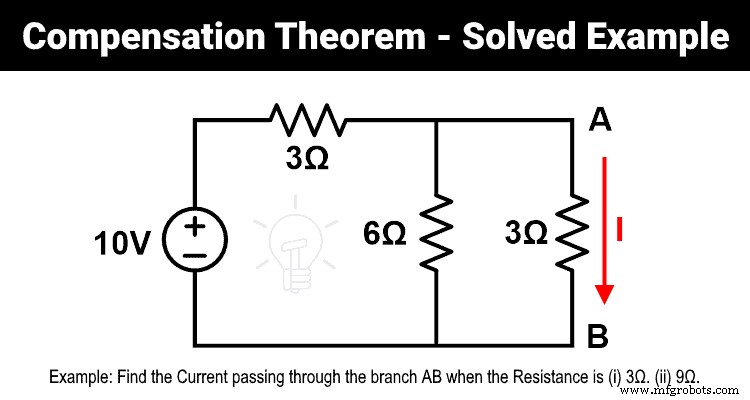
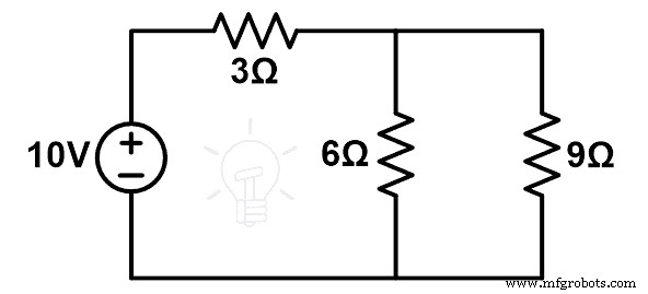
Example-1

• 1) Find the current passing through the branch AB when the resistance is 3Ω.
• 2) Find the current passing through the branch AB using compensation theorem when the 3Ω resistance is changed to 9Ω.
• 3) Prove compensation theorem.

Answer-1

As shown in the figure, the 6Ω and 3Ω resistors are in parallel. And this parallel combination is connected in series with 3Ω resister. Therefore, equivalent resistance will be;

R_Eq = 6 | | 3+3

 

 

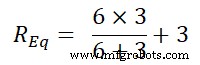
R_Eq = 2 + 3

R_Eq = 5 Ω

According to Ohm’s law;

10 = I (5)

I = 10 ÷ 5

I = 2 A

Now, we need to find the current passes through branch AB. So, according to the current divider rule;

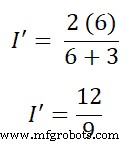
I’ = 1.333 A (or 3/4 A)

• Related Post: Substitution Theorem – Step by Step Guide with Solved Example

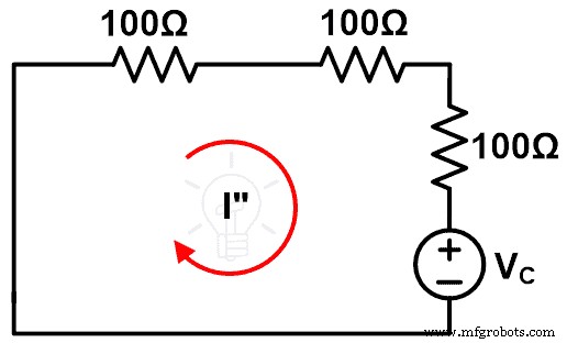
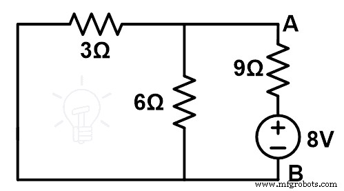
Answer-2

We need to replace the 3Ω resister with a 9Ω resister. According to the compensation theorem, we need to add a new voltage source in series with the 9Ω resister. And the value of this voltage source is;

V_C = I’ ΔZ

Where,

ΔZ = 9 – 3 = 6 Ω and I’ = 4/3 A (or 1.333 A)

V_C = (4/3A) x 6 Ω

V_C = 8 V

A modified circuit diagram or compensated circuit diagram is as shown in the below figure.

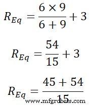
Now, we will find the equivalent resistance. Here, 3Ω and 6Ω resistors are connected in parallel. And this parallel combination is connected in series with a 9Ω resister.

R_Eq = 3 | | 6 + 9

R_Eq = 2 + 9

R_Eq = 11 Ω

Now, according to Ohm’s law;

V = ΔI R

8 = ΔI (11 Ω)

ΔI = 8 ÷ 11

ΔI = 0.7272 A

So, according to the compensation theorem; the change in current is 0.7272A.

• Related Post: Tellegen’s Theorem – Solved Examples & MATLAB Simulation

Answer-3

We want to prove the compensation theorem. So, we calculate the current in the given example with a 9Ω resister.

The modified circuit diagram is shown in the figure below.

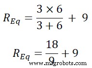
Here, 9Ω and 6Ω resistors are connected in parallel and this parallel combination is connected in series with the 3Ω resister.

The equivalent resistance is equal to;

R_Eq = 9 | | 6 + 3

R_Eq = 99 ÷ 15

R_Eq = 6.66 Ω

From the above figure;

10 = I (6.66)

I = 10 ÷ 6.66

I = 1.5151 A

According to the current divider rule;

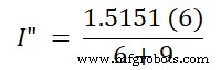
I” = 0.6060A

ΔI = I’ – I”

ΔI = (4/3A) – 0.6060

ΔI = 1.333A – 0.6060

ΔI = 0.7273 A

Hence, it is proved that the change in current calculate from the compensation theorem is the same as the change in current calculated from the original circuit.

• Related Post: Maximum Power Transfer Theorem for AC & DC Circuits
  

Example-2

In the below circuit, find the change of current if 3Ω resister is replaced by a 7Ω resister using compensation theorem. And prove the compensation theorem.

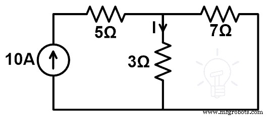
The above network consists of only resistors and independent current sources. So, we can apply the compensation theorem to this network.

In this figure, the network is supplied by a current source. Now, we need to find the current that passes through the 3Ω resister branch. This current can be found using KCL or KVL. But here, this current can easily find by the current divider rule.

Therefore, according to the current divider rule;

I = 70 ÷ 10 A

I = 7 A

In the original network with 3Ω resister, the current that passes through that branch is 3A. Now, we need to change this resister from 3Ω to 7Ω. Due to this modification, the current passes through that branch will be changed. And we will find this change of current by compensation theorem.

For that, we need to make a compensation network. To make a compensation network, we need to remove all independent sources available in the network by short-circuiting the voltage source and open-circuiting the current source.

In this network, only one current source is available. We assume the current source is an ideal current source. Therefore, we do not require to add the internal resistance.

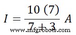
The second modification we need to make in the compensation circuit is to add an extra voltage source. And the value of this voltage is;

V_C = I ΔZ

V_C = 7 × (7 – 3)

V_C = 7 × 4

V_C = 28 V

The compensation network is as shown in the figure below.

This figure has only one loop. And the current that passes through the branch of 7Ω will give us the change of current (∆I).

ΔI = V_C ÷ (7+7)

ΔI = 28 ÷ 14

ΔI = 2 A

To prove the compensation theorem, we will find the current in the circuit with a 7Ω resistor connected. The modified circuit diagram is shown in the figure below.

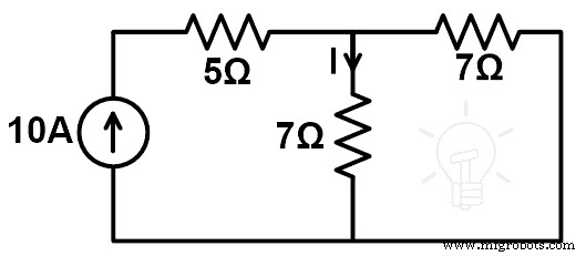
I” = (10 (7)) ÷ (7 + 7)

I” = 70 ÷ 14

I” = 5 A

By applying the current divider rule;

To find the change of current, we need to subtract this current from the current that passes through the original network.

ΔI = I – I”

ΔI = 7 – 5

ΔI = 2 A

Hence, we have proved the compensation theorem.

Related Electric Circuit Analysis Tutorials:

• SUPERNODE Circuit Analysis – Step by Step with Solved Example
• SUPERMESH Circuit Analysis – Step by Step with Solved Example
• Kirchhoff’s Current & Voltage Law (KCL & KVL) | Solved Example
• Cramer’s Rule Calculator – 2 and 3 Equations System for Electric Circuits
• Wheatstone Bridge – Circuit, Working, Derivation and Applications
• Electrical and Electronics Engineering Calculators
• 5000+ Electrical and Electronic Engineering Formulas & Equations