Training Neural Networks with Excel: Building & Validating a Python Multilayer Perceptron

In this article, we’ll show how to generate training data in Excel, train a multilayer perceptron in Python, and validate its performance.

If you’re looking to develop a Python neural network, you’re in the right place. Before diving into the Excel‑based data preparation, consider reviewing the rest of the series below for foundational context:

1. How to Perform Classification Using a Neural Network: What Is the Perceptron?
2. How to Use a Simple Perceptron Neural Network Example to Classify Data
3. How to Train a Basic Perceptron Neural Network
4. Understanding Simple Neural Network Training
5. An Introduction to Training Theory for Neural Networks
6. Understanding Learning Rate in Neural Networks
7. Advanced Machine Learning with the Multilayer Perceptron
8. The Sigmoid Activation Function: Activation in Multilayer Perceptron Neural Networks
9. How to Train a Multilayer Perceptron Neural Network
10. Understanding Training Formulas and Backpropagation for Multilayer Perceptrons
11. Neural Network Architecture for a Python Implementation
12. How to Create a Multilayer Perceptron Neural Network in Python
13. Signal Processing Using Neural Networks: Validation in Neural Network Design
14. Training Datasets for Neural Networks: How to Train and Validate a Python Neural Network

What Is Training Data?

In real‑world applications, training samples consist of measured inputs paired with known targets that enable a neural network to learn a consistent input‑output mapping. For example, suppose you want a network to predict the eating quality of a tomato based on color, shape, and density. By collecting thousands of tomatoes, recording their physical attributes, tasting each one, and compiling the results into a table, you create the dataset that the network will use to learn the relationship between attributes and quality.

Each row represents one training sample with three input columns (color, shape, density) and a single target output column.

 

During training, the neural network will identify the underlying pattern—if one exists—between the three input values and the output value.

Quantifying Training Data

All inputs and outputs must be numerical. Strings such as "plum‑shaped" or "mouthwatering" cannot be fed directly into the network. Quantization converts qualitative descriptors into numeric scales. For instance, shape could be encoded from –1 (perfect sphere) to +1 (extremely elongated). Eating quality could be rated on a five‑point scale and then one‑hot encoded into a five‑element output vector.

The following diagram illustrates one‑hot encoding for a five‑class classification task.

 

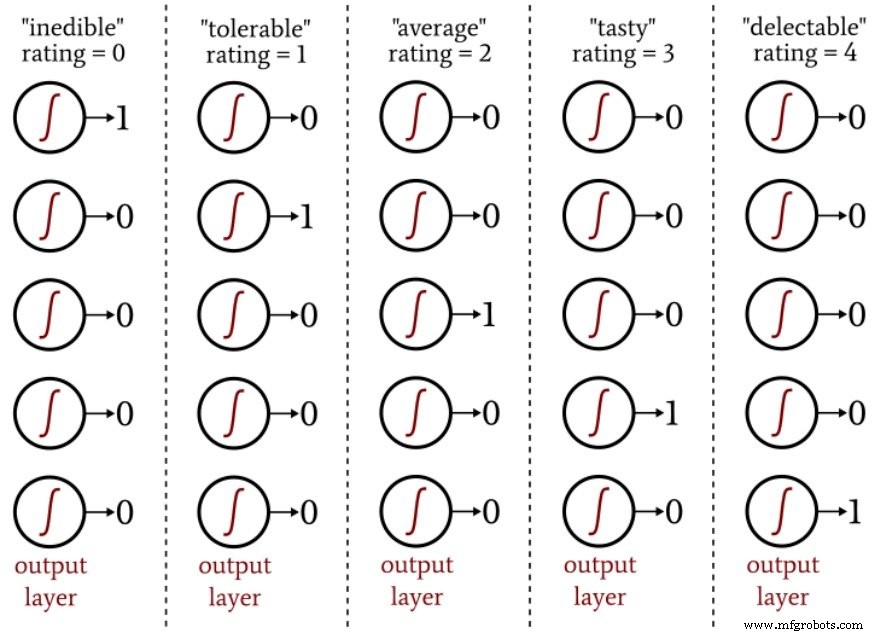
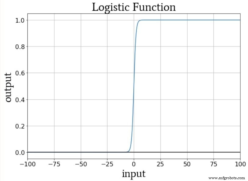
One‑hot encoding aligns well with logistic‑sigmoid activation, which produces values close to 0 or 1 outside a narrow transition zone. Using a single output node with target values 0–4 would bias the network toward the extremes and lead to nonsensical predictions.

Creating a Training Data Set

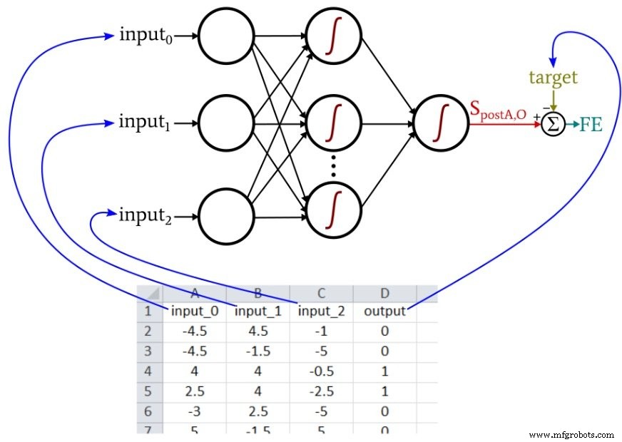
The Python neural network referenced in Part 12 imports samples from an Excel file. The data used here are arranged as follows:

 

Because our Perceptron implementation supports only a single output node, we perform a binary classification. The input values are random numbers between –5 and +5, generated with this Excel formula:

=RANDBETWEEN(-10, 10)/2

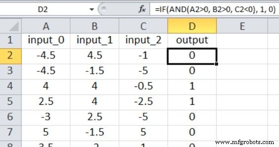
The output is derived from the following rule:

=IF(AND(A2>0, B2>0, C2<0), 1, 0)

Thus, the network learns that a sample is labeled 1 only when input_0 > 0, input_1 > 0, and input_2 < 0; otherwise, it receives a 0.

For this simple problem, 5,000 randomly generated samples and a single epoch are sufficient to achieve high classification accuracy.

Training the Network

Configure the network with an input dimensionality of three (I_dim = 3), four hidden nodes (H_dim = 4), and a learning rate of 0.1 (LR = 0.1). Replace the training_data = pandas.read_excel(...) line with the path to your spreadsheet. If you lack Excel, Pandas can also read ODS files.

Running the training script on a 2.5 GHz Windows laptop with 5,000 samples completes in just a few seconds. If you’re using the full MLP_v1.py script, validation will automatically begin after training.

Validating the Network

Validation requires a second spreadsheet generated with the same formulas. Import this data in the same way as the training data:

 

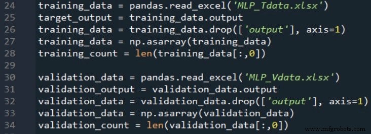
The following snippet demonstrates a straightforward validation routine:

# Feed‑forward to obtain post‑activation value
output = sigmoid(np.dot(W_out, hidden_output))
# Apply threshold to obtain binary prediction
prediction = 1 if output > 0.5 else 0
# Compare with target and accumulate correct predictions

Classification accuracy is calculated by dividing the number of correct predictions by the total number of validation samples.

If np.random.seed(1) is omitted, weight initialization will vary between runs, causing accuracy to fluctuate. Across 15 runs with the specified parameters (5,000 training samples, 1,000 validation samples), accuracy ranged from 88.5% to 98.1%, averaging 94.4%.

Conclusion

We explored key concepts behind neural‑network training data, implemented a Python multilayer Perceptron, and evaluated its performance using Excel‑generated datasets. The series has progressed significantly from its inception, and many more advanced topics await in upcoming posts.