Training a Basic Perceptron Neural Network with Python: Step‑by‑Step Guide

Training a Basic Perceptron Neural Network with Python

This guide walks you through a fully commented Python implementation that automatically learns the weights for a single‑layer perceptron. The code is ready to copy‑paste, run, and adapt to your own data.

Explore the AAC Perceptron Series

For deeper context or to jump into advanced topics, check out the rest of our articles:

1. How to Perform Classification Using a Neural Network: What Is the Perceptron?
2. How to Use a Simple Perceptron Neural Network Example to Classify Data
3. How to Train a Basic Perceptron Neural Network
4. Understanding Simple Neural Network Training
5. An Introduction to Training Theory for Neural Networks
6. Understanding Learning Rate in Neural Networks
7. Advanced Machine Learning with the Multilayer Perceptron
8. The Sigmoid Activation Function: Activation in Multilayer Perceptron Neural Networks
9. How to Train a Multilayer Perceptron Neural Network
10. Understanding Training Formulas and Backpropagation for Multilayer Perceptrons
11. Neural Network Architecture for a Python Implementation
12. How to Create a Multilayer Perceptron Neural Network in Python
13. Signal Processing Using Neural Networks: Validation in Neural Network Design
14. Training Datasets for Neural Networks: How to Train and Validate a Python Neural Network

Classification with a Single‑Layer Perceptron

We begin with a classic binary classification problem in 3‑D space. The network’s architecture is a single hidden layer with three input nodes and one output node that uses a unit‑step activation function.

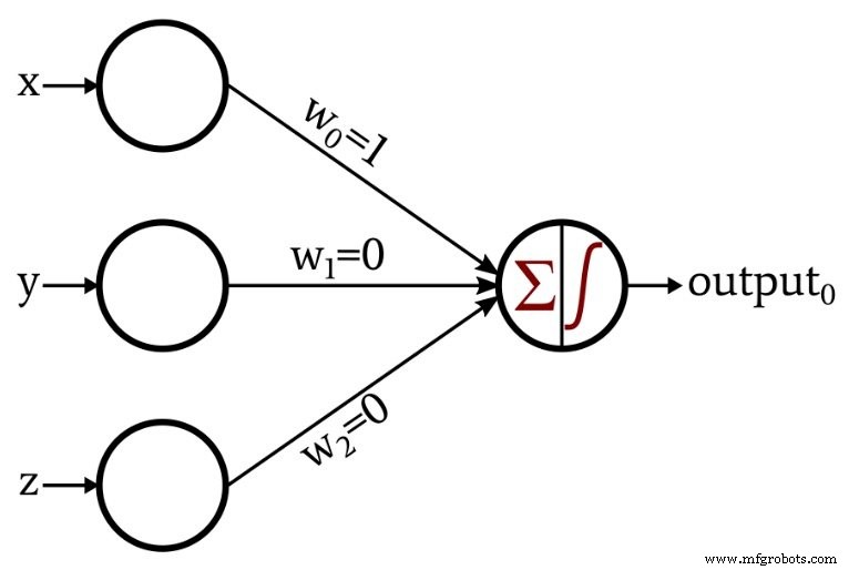
The output node applies the following unit‑step function:

\[f(x)=\begin{cases}0 & x < 0\\1 & x \ge 0\end{cases}\]

To illustrate learning, we extend the architecture to automatically adjust its weights via a simple training loop:

A Python Implementation

The following script reads training data from an Excel file, initializes weights randomly, and iteratively updates them using the perceptron learning rule.

import pandas
import numpy as np

# Dimensionality of input space (x, y, z)
input_dim = 3

# Learning rate controls weight adjustment magnitude
learning_rate = 0.01

# Random initial weights; you can set fixed values for reproducibility
Weights = np.random.rand(input_dim)
# Weights = np.array([0.5, 0.5, 0.5])

# Load dataset: a sheet with columns for each feature and an 'output' column
Training_Data = pandas.read_excel("3D_data.xlsx")

# Separate expected outputs from the feature matrix
Expected_Output = Training_Data.output
Training_Data = Training_Data.drop(["output"], axis=1)

# Convert to NumPy array for vectorized operations
Training_Data = np.asarray(Training_Data)
training_count = len(Training_Data[:, 0])

# Train over multiple epochs
for epoch in range(5):
    for datum in range(training_count):
        # Weighted sum of inputs
        Output_Sum = np.sum(np.multiply(Training_Data[datum, :], Weights))

        # Apply unit‑step activation
        Output_Value = 0 if Output_Sum < 0 else 1

        # Compute error between expected and actual output
        error = Expected_Output[datum] - Output_Value

        # Update each weight according to the learning rule
        for n in range(input_dim):
            Weights[n] += learning_rate * error * Training_Data[datum, n]

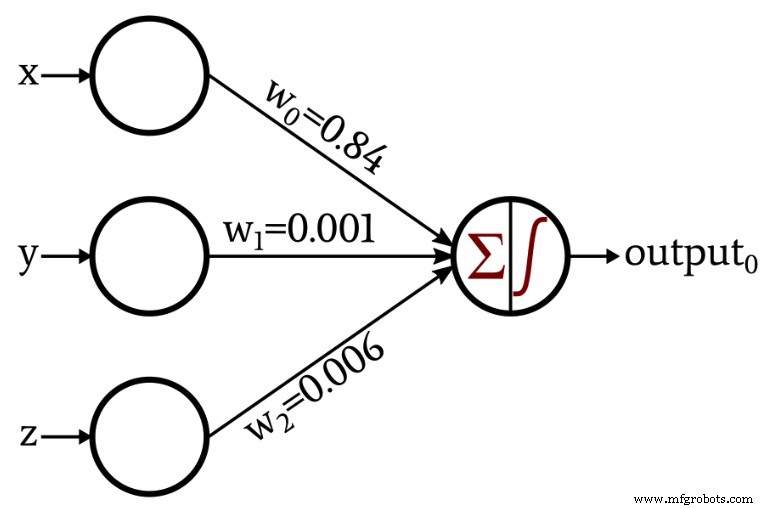
print(f"w_0 = {Weights[0]:.3f}")
print(f"w_1 = {Weights[1]:.3f}")
print(f"w_2 = {Weights[2]:.3f}")

Key Concepts Explained

Configuring the Network and Organizing Data

The network has three input nodes to match the 3‑D coordinates. The learning rate of 0.01 is a standard starting point; you may adjust it after experimentation. Weights are seeded randomly to avoid symmetry, but you can set them to a fixed value if you want deterministic behavior.

Training data is read from an Excel file, split into inputs and expected outputs, and then converted to a NumPy array for efficient computation.

Calculating Output Values

Each epoch iterates over all training samples. For each sample, the weighted sum of the inputs is computed. The unit‑step function then maps this sum to a binary output: 0 if the sum is negative, 1 otherwise.

Updating Weights

When the predicted output differs from the expected output, the perceptron learning rule adjusts each weight proportionally to the input value, the error, and the learning rate:

\[w_{new} = w + (\alpha \times \delta \times input)\]

where \(\delta = \text{output}_{expected} - \text{output}_{calculated}\) and \(\alpha\) is the learning rate.

Conclusion

You've now seen a complete, annotated implementation of a single‑layer perceptron in Python. The code is a solid foundation for experimenting with different datasets, learning rates, or even extending the network to multiple outputs in future projects.