Mastering Electric Circuit Simulation with SPICE: A Practical Guide for Designers and Students

When harnessed correctly, computers become indispensable allies in science and engineering. One of the most powerful applications is the simulation of electric circuits. These programs enable designers to evaluate concepts quickly, reducing both time and expense compared to physical prototyping.

For students beginning in electronics, simulation offers an immediate, hands‑on way to experiment with circuit behavior without assembling hardware. While real‑world testing remains essential, virtual experiments help build intuition and allow rapid iteration.

Throughout this guide, I’ll intersperse SPICE simulation screenshots to illustrate key concepts. By studying these results, learners can grasp circuit dynamics without getting bogged down in complex mathematics.

Circuit Simulation with SPICE

To model circuits on a computer, I use SPICE (Simulation Program with Integrated Circuit Emphasis). SPICE interprets a textual description of a circuit—called a netlist—and outputs the results of a detailed mathematical analysis.

For those interested in deeper details, Volume 5 of this series’ reference section covers SPICE comprehensively. Here, I’ll focus on the fundamentals and walk through simple examples.

First, SPICE must be installed on your machine. It is freely available for many operating systems, and I’ll demonstrate with the lightweight version 2G6, chosen for its ease of use.

Next, let’s analyze a basic circuit shown earlier: a 10‑volt battery in series with a 5‑Ω resistor. The goal is to verify that SPICE calculates the expected current using Ohm’s Law (I = E / R).

SPICE is a Text‑Based Program

SPICE does not interpret graphical schematics; it requires a purely textual description. Each unique connection point is assigned a node number. Nodes that share a common point are given the same number. SPICE also expects a node 0 to serve as the reference (ground).

In our simple example we only have two nodes—node 1 and node 0:

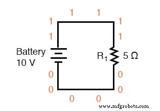
Although this diagram illustrates node numbering, SPICE demands the same information in plain text.

Creating SPICE Netlists with a Text Editor

A text editor—such as Notepad on Windows or Vim on Linux—provides a clean, formatting‑free environment to write netlists. SPICE relies on the exact syntax of these files.

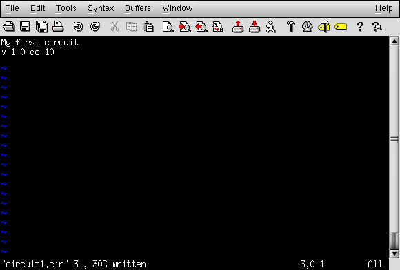
Begin by adding a title line:

Define the voltage source with the letter “v”, the node numbers, and the DC voltage value:

Then specify the resistor using “r” and its node connections:

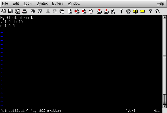
Close the netlist with an .end statement. The complete netlist looks like this:

Running SPICE from the Command Line

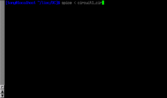
After saving the file—e.g., as circuit1.cir—invoke SPICE from a terminal:

spice < circuit1.cir

On a Linux system, the command line before pressing Enter appears as follows:

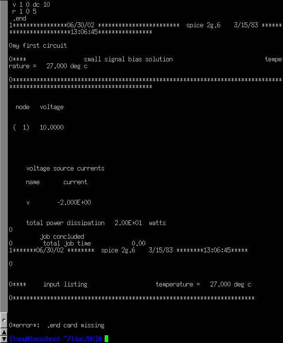
SPICE then prints its netlist, node voltages, source currents, and total power dissipation. The output for our example is:

Note that SPICE reports the current as a negative value due to its internal sign convention. The power is displayed in scientific notation (2.00E+01 W).

Redirecting Output to a Text File

To suppress screen output and capture the results in a file, redirect SPICE’s output:

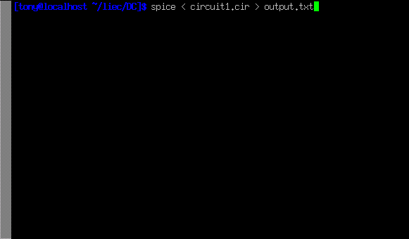
The resulting file—output1.txt—can be edited with a text editor. After removing extraneous headers, the core data remains ready for analysis or inclusion in documents:

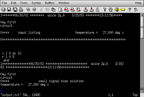
Here is the cleaned‑up output presented directly in text form:

my first circuit 
 v 1 0 dc 10 
 r 1 0 5 
 .end
 node voltage
 ( 1) 10.0000
 voltage source currents
 name current
 v -2.000E+00
 total power dissipation 2.00E+01 watts

Altering Component Values

To change a component, edit the netlist, save it, and rerun SPICE. For example, tripling the voltage to 30 V yields the following results:

second example circuit 
 v 1 0 dc 30
 r 1 0 5
 .end
 node voltage
 ( 1) 30.0000
 voltage source currents
 name current
 v -6.000E+00
 total power dissipation 1.80E+02 watts

The current increased from 2 A to 6 A, and power rose ninefold—from 20 W to 180 W—consistent with Joule’s Law (P = E² / R).

Using SPICE Sweep and Plot Features

To examine the circuit over a voltage range, add a .dc directive. Comments—lines beginning with “*”—help document the netlist:

third example circuit
 v 1 0
 r 1 0 5
 *the ".dc" statement tells spice to sweep the "v" supply
 *voltage from 0 to 100 volts in 5 volt steps.
 .dc v 0 100 5
 .print dc v(1) i(v)
 .end

The .print command outputs tabular data for each step:

v i(v) 
 0.000E+00 0.000E+00
 5.000E+00 -1.000E+00
 1.000E+01 -2.000E+00
 1.500E+01 -3.000E+00
 2.000E+01 -4.000E+00
 2.500E+01 -5.000E+00
 3.000E+01 -6.000E+00
 3.500E+01 -7.000E+00
 4.000E+01 -8.000E+00
 4.500E+01 -9.000E+00
 5.000E+01 -1.000E+01
 5.500E+01 -1.100E+01
 6.000E+01 -1.200E+01
 6.500E+01 -1.300E+01
 7.000E+01 -1.400E+01
 7.500E+01 -1.500E+01
 8.000E+01 -1.600E+01
 8.500E+01 -1.700E+01
 9.000E+01 -1.800E+01
 9.500E+01 -1.900E+01
 1.000E+02 -2.000E+01

Changing .print to .plot generates a simple text‑based graph:

Legend: + = v#branch 
 ------------------------------------------------------------------------
 sweep v#branch-2.00e+01 -1.00e+01 0.00e+00
 ---------------------|------------------------|------------------------|
 0.000e+00 0.000e+00 . . +
 5.000e+00 -1.000e+00 . . + .
 1.000e+01 -2.000e+00 . . + .
 1.500e+01 -3.000e+00 . . + .
 2.000e+01 -4.000e+00 . . + .
 2.500e+01 -5.000e+00 . . + .
 3.000e+01 -6.000e+00 . . + .
 3.500e+01 -7.000e+00 . . + .
 4.000e+01 -8.000e+00 . . + .
 4.500e+01 -9.000e+00 . . + .
 5.000e+01 -1.000e+01 . + .
 5.500e+01 -1.100e+01 . + . .
 6.000e+01 -1.200e+01 . + . .
 6.500e+01 -1.300e+01 . + . .
 7.000e+01 -1.400e+01 . + . .
 7.500e+01 -1.500e+01 . + . .
 8.000e+01 -1.600e+01 . + . .
 8.500e+01 -1.700e+01 . + . .
 9.000e+01 -1.800e+01 . + . .
 9.500e+01 -1.900e+01 . + . .
 1.000e+02 -2.000e+01 + . .
 ---------------------|------------------------|------------------------|
 sweep v#branch-2.00e+01 -1.00e+01 0.00e+00

Interpreting SPICE Output with External Tools

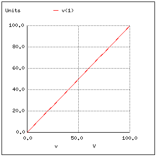
Graphical programs such as Nutmeg can read SPICE’s text output and plot the data visually. A typical Nutmeg plot displays the resistor voltage (v(1)) increasing linearly with the applied source voltage.

Regardless of how proficient you become with SPICE, understanding the numbers in its reports is essential. I’ll continue to annotate output in forthcoming examples to demystify the results and unlock the tool’s full potential.

RELATED WORKSHEETS:

• Basic Electricity Worksheet
• Basic DC Worksheet
• Basic Network Analysis Worksheet
• Basic AC Worksheet
• Basic Semiconductor Worksheet
• Basic Analog Circuit Worksheet
• Basic Digital Circuit Worksheet