Parallel Tank Circuit Resonance: Theory, Calculations, and SPICE Verification

Resonance in a Parallel Tank Circuit

In a parallel LC (tank) circuit, resonance is achieved when the inductive reactance (ÅXL = 2πfL) exactly equals the capacitive reactance (ÅXC = 1/(2πfC)). Because inductive reactance rises with frequency while capacitive reactance falls, only one frequency satisfies this balance.

Example:

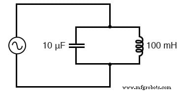
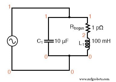
Simple parallel resonant circuit (tank circuit).

For the circuit shown, we have a 10 µF capacitor and a 100 mH inductor. By setting the two reactance formulas equal and solving for frequency, we obtain the resonant frequency:

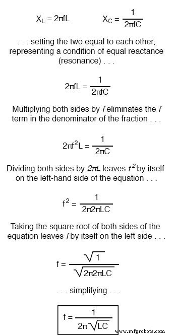
This yields a resonant frequency of 159.155 Hz when L = 100 mH and C = 10 µF.

Calculating Individual Impedances

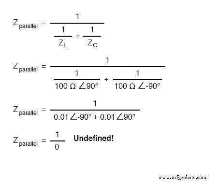
At resonance, the equal and opposite reactances cancel each other out, causing the total impedance of the parallel LC pair to approach infinity. In practical terms, the tank circuit behaves like an open circuit and draws negligible current from the AC source.

To illustrate this, we can compute the individual impedances of the 10 µF capacitor and 100 mH inductor and apply the parallel impedance formula:

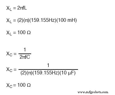
These component values were chosen to produce resonant impedances that are easy to work with (100 Ω).

Parallel Impedance Formula

Using the standard parallel impedance expression, we confirm that the total impedance diverges as the reactances converge:

SPICE Simulation Overview

Although a mathematical division by zero is undefined, the SPICE model demonstrates that the total impedance tends toward infinity as the frequency nears resonance. We simulate the circuit across a wide frequency range to observe this behavior.

Resonant Circuit for SPICE Simulation

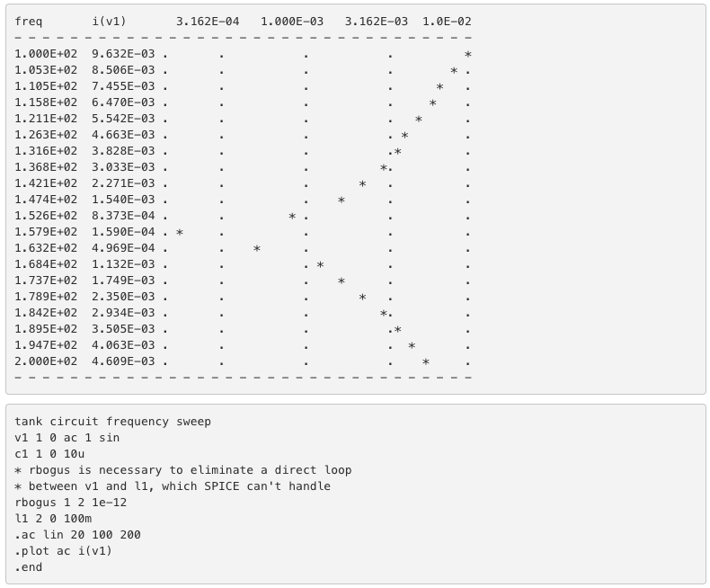
Because SPICE cannot analyze a loop containing a purely inductive source, a 1 pΩ resistor is inserted to provide a minimal, non‑intrusive path for current flow. The resulting current plot shows a sharp dip near the predicted resonance of 159.155 Hz.

Nutmeg Post‑Processor Plot

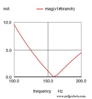
While the raw .plot command produces a text output, the Nutmeg graphical post‑processor yields a clearer visual of the current magnitude versus frequency:

spice -b -r resonant.raw resonant.cir
nutmeg resonant.raw

From the Nutmeg prompt:

>setplot ac1
>display
>plot mag(v1#branch)

Bode Plots

These SPICE outputs are a form of Bode plot, which graphically represent amplitude (or phase) versus frequency. The steepness of the curve indicates how sharply the circuit responds to frequency changes.

Key Takeaways

• Resonance occurs when ÅXL equals ÅXC.
• For an ideal, resistanceless tank circuit, the resonant frequency is f₀ = 1/(2π√LC).
• At resonance, the parallel LC’s total impedance approaches infinity, effectively acting as an open circuit.
• A Bode plot visualizes the circuit’s frequency response, showing amplitude or phase versus frequency.

Related Worksheets

• Fundamentals of Radio Communication Worksheet
• Resonance Worksheet