Analog vs. Digital Computational Circuits: A Practical Guide

When the word “computer” comes up, most people picture a digital device that processes information in binary—discrete 1’s and 0’s—using countless transistors that toggle between saturation and cutoff. Yet analog circuitry can represent and manipulate numerical values with continuous voltage signals, enabling real‑time mathematical operations.

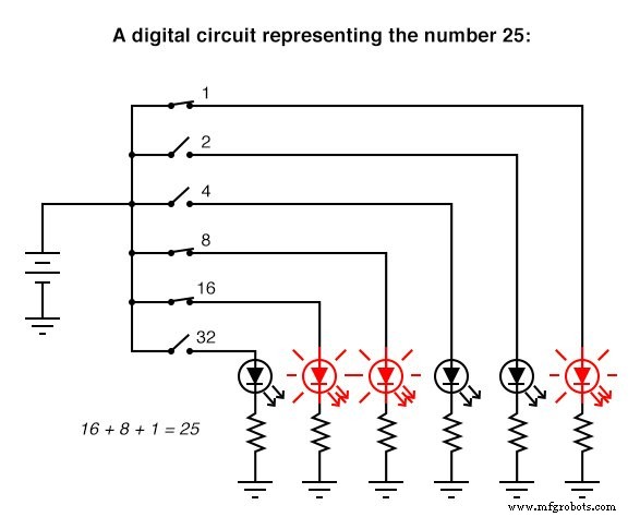
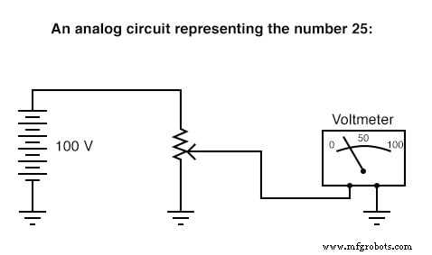
Below is a straightforward illustration of the same number, “twenty‑five”, encoded in binary versus an analog voltage.

Digital computational circuits are inherently more complex than their analog counterparts. They often require a sequence of logic stages—much like a human solving a problem step by step—to arrive at a final answer. In contrast, analog circuits perform calculations continuously and instantaneously, though they suffer from imprecision due to drift and noise.

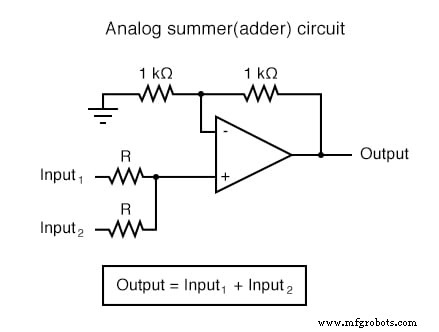
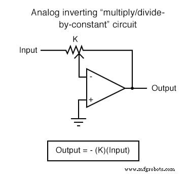
Where exactness is not paramount, analog computational circuits offer a clean, component‑efficient solution. Below are a few common op‑amp topologies that perform elementary mathematical functions.

Computational Op‑Amp Circuits

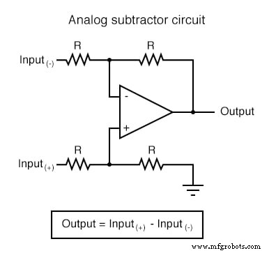
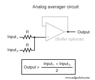
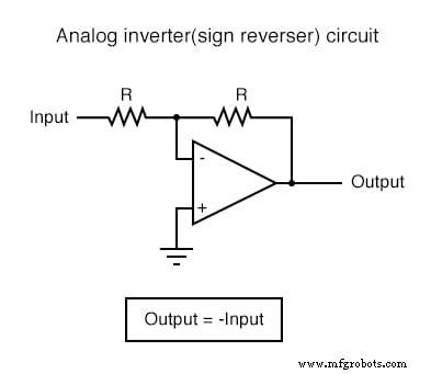
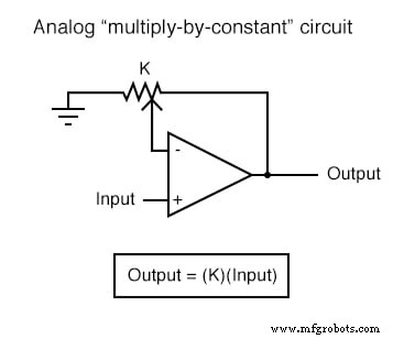
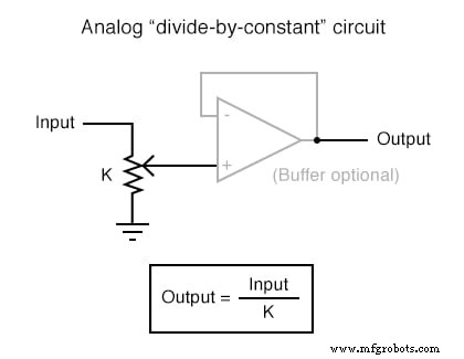
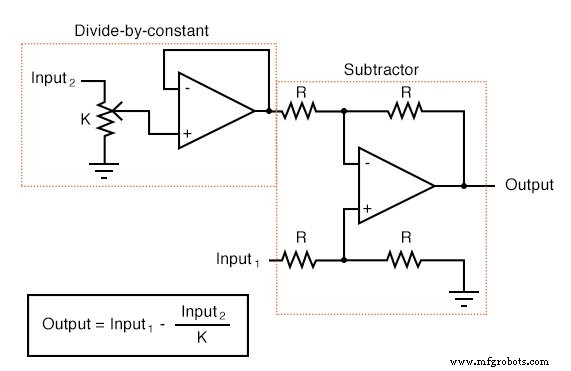
By wiring these modules together, designers can build complex systems. For instance, a circuit that subtracts a fraction of one variable from another can be assembled from a divide‑by‑constant block followed by a subtractor, as shown below.

Historically, analog computers—composed of these very op‑amp networks—were staples in academia and industry for modeling mathematical equations. While digital computers have largely replaced them, the elegance and minimal component count of analog computational circuitry remain unmatched in certain applications.

Analog circuits excel at the calculus operations of integration and differentiation. These functions are achieved by exploiting the voltage‑time relationship of a capacitor within an op‑amp feedback loop. To fully appreciate their operation, it is helpful to revisit the underlying calculus concepts.

As John I. Smith notes in Modern Operational Circuit Design:

“Integral calculus is one of the mathematical disciplines that operational [amplifier] circuitry exploits and, in the process, rather demolishes as a barrier to understanding.” (pg. 4)

Engineer George Fox Lang echoed this sentiment in his 2000 article for Sound and Vibration, stating:

“Creating a real physical entity (a circuit) governed by a particular set of equations and interacting with it provides unique insight into those mathematical statements. There is no better way to develop a “gut feel” for the interplay between physics and mathematics than to experience such an interaction. The analog computer was a powerful interdisciplinary teaching tool; its obsolescence is mourned by many educators in a variety of fields.” (pg. 23)

Students first learn differentiation, the instantaneous rate of change of one variable with respect to another. In an analog differentiator, time is the independent variable, so the output represents how quickly a voltage signal changes over time.

Consider a car traveling in a straight line. Its position, x, plotted against time, t, yields a straight line if the speed is constant:

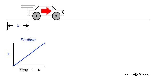
Differentiating position with respect to time gives velocity: dx/dt (shown as a flat line). The slope of the position graph directly translates to the derivative.

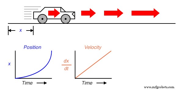
If the car’s distance grows exponentially, the velocity increases over time, producing a rising line for dx/dt:

The differentiator’s output voltage is proportional to the slope of the input signal, as illustrated in the following circuit.

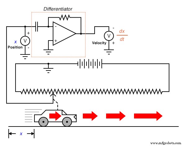
Because the differentiator is inverting, the voltmeter must be wired in reverse polarity to display a positive velocity value.

Symbolic differentiation requires a known mathematical expression. For example, the derivative of y = 3x is 3, and the derivative of y = 3x² is 6x. However, most real‑world signals cannot be described by a simple formula, making symbolic methods impractical. Analog differentiators solve this by physically computing the rate of change for any input waveform.

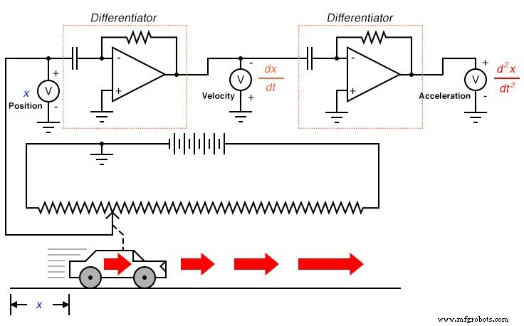
Applying a second differentiator yields acceleration (the rate of change of velocity), as depicted below.

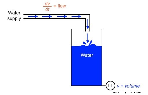
These principles extend beyond motion. For instance, a level transmitter on a water tank produces a voltage proportional to volume. Differentiating this signal provides the flow rate into the tank.

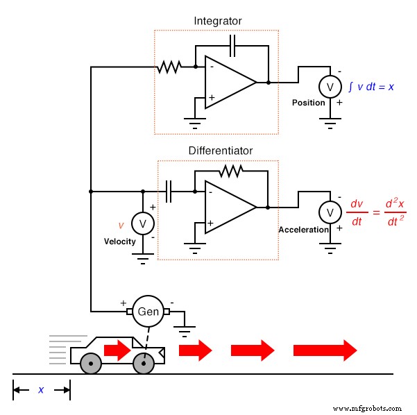
Conversely, an integrator circuit performs the inverse operation—accumulating a signal over time. An integrator fed by a velocity signal from a tachogenerator will produce a voltage proportional to distance traveled.

Integration inherently averages high‑frequency noise, acting as a low‑pass filter. This contrasts with differentiation, which amplifies noise due to its reliance on rapid voltage changes.

However, integrators introduce their own challenges. The continuous accumulation of input bias currents and leakage in capacitors causes output drift, while sensor offsets can lead to cumulative error. These artifacts are distinct from the mathematical properties of integration, which always yields an arbitrary constant of integration.

In practice, the most accurate measurement is achieved by directly sensing the desired variable. Computation remains invaluable when direct measurement is impossible, but engineers must understand the limits and error sources inherent to analog processing.

RELATED WORKSHEET:

• Linear Computational Circuitry Worksheet