Understanding Mutual Inductance and Transformer Fundamentals

Behaviors of Inductors Wrapped Around a Conductive Core

Imagine winding insulated copper wire around a ferromagnetic loop and energizing it with an AC source. The resulting iron‑core coil presents an inductive reactance that limits the AC current, just as any inductor does:

X_L = 2πfL and I = E/X (or I = E/Z)

To fully grasp the device’s operation, we must examine how voltage, current, and magnetic flux interact.

Kirchhoff’s voltage law dictates that the algebraic sum of all voltages around a loop is zero. In a single‑source, single‑load circuit, the voltage drop across the load must equal the source voltage, assuming negligible wire resistance.

Thus, the inductor must generate an opposing voltage that matches the source in magnitude but opposes it in phase. For a resistor, this opposing voltage stems from electrical energy dissipation. For an ideal inductor (no wire resistance), the opposition comes from the changing magnetic flux in the iron core, which induces a counter‑EMF according to Faraday’s law.

Relationship Between Voltage, Current and Magnetic Flux

Faraday discovered that the instantaneous voltage across a coil equals the number of turns (N) multiplied by the instantaneous rate of change of magnetic flux (dΦ/dt):

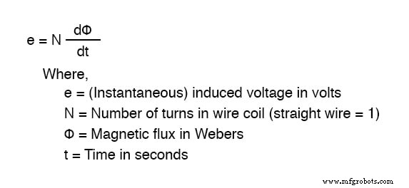
This relationship produces sine‑wave voltages when driven by a sinusoidal source, with the flux wave lagging the voltage by 90°:

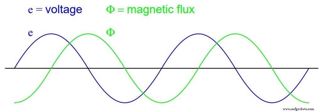
Because the induced voltage must counteract the applied voltage, the AC current in an iron‑core inductor lags the voltage by 90°. This current, often called the magnetizing current, is the coil’s effort to produce the necessary magnetic flux.

In practice, the magnetizing current is not perfectly sinusoidal because of the nonlinear B/H curve of iron. If the core approaches saturation, the flux density rises sharply, and the current waveform distorts into a bell‑shaped shape:

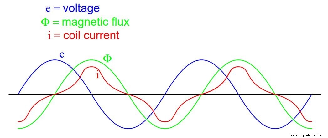
When saturation occurs, disproportionately larger magnetomotive force (MMF) is required for each incremental increase in flux. Since MMF is proportional to current (MMF = NI), the coil current spikes during the peaks of the cycle, creating the observed distortion.

Exciting Current and Its Effects

Core losses—hysteresis and eddy currents—add further distortion and slightly advance the phase of the current relative to the voltage. The combined current that includes magnetization and loss components is known as the exciting current.

Minimizing this distortion typically requires operating at low flux densities, which in turn demands a core with a larger cross‑sectional area, making the inductor bulkier and more expensive.

For simplicity, we’ll assume an ideal, loss‑free core far from saturation, resulting in a purely sinusoidal exciting current. Such a coil exchanges energy alternately with the source but dissipates no power in a perfect scenario.

Introducing a Second Coil: Mutual Induction

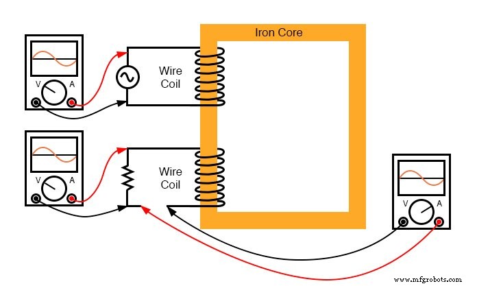
Now add a second coil wound around the same iron core. The first coil, energized by the AC source, is the primary; the second, initially open, is the secondary:

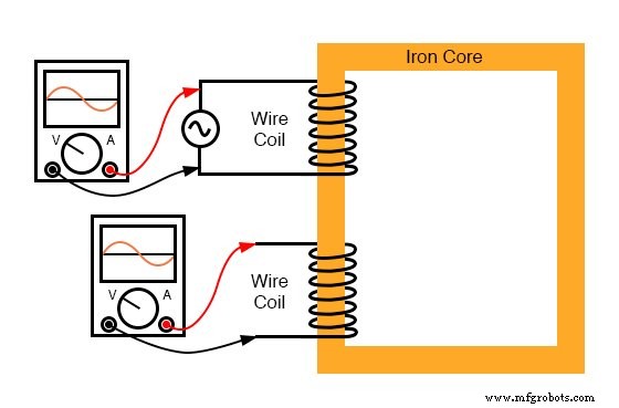
If the secondary experiences the same flux change as the primary and has an identical turn count, it will see an induced voltage of equal magnitude and phase to the primary voltage:

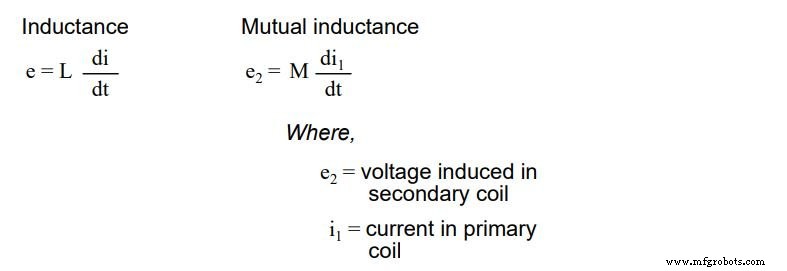
This phenomenon is called mutual inductance, measured in henries but denoted by the capital letter “M.”

With the secondary open, no current flows. However, connecting a resistive load allows current to flow in phase with the induced voltage, as the voltage across a resistor is always in phase with its current:

While one might expect the secondary current to alter the core flux, it does not. The primary’s induced voltage must remain balanced with the source voltage, enforcing a constant flux. The secondary’s MMF is instead counteracted by an equal but opposite MMF generated in the primary, maintaining flux equilibrium.

Thus, the secondary’s load current is “reflected” to the primary, drawing current from the source as if the load were directly connected to the primary supply.

From Mutual Inductance to Transformers

In this arrangement, the primary acts as a load to the source, while the secondary behaves as a source to the load. The transformer’s role is to convert electrical energy to magnetic energy and back, enabling power transfer without direct electrical connection.

Transformers are inherently AC devices because they rely on changing magnetic flux. Their schematic symbol consists of two inductors sharing a common core:

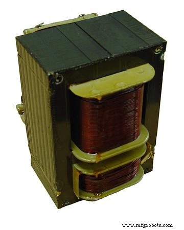
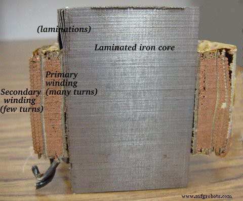
Typical transformers use ferromagnetic cores, but air‑cored versions exist. A practical example is the gas‑discharge lighting transformer shown below:

Primary and Secondary Windings

Each winding is simply a coil of insulated wire. The top coil usually has more turns and carries a thicker wire than the bottom coil, reflecting the differing voltage and current requirements of the primary and secondary.

Cut‑away images reveal the core’s laminated structure, which reduces eddy current losses:

Simulating a Transformer with SPICE

Transformers can be modeled in SPICE as two coupled inductors. The coupling coefficient (k) describes how closely the inductors are magnetically linked; a value of 1.0 represents perfect coupling.

Below is a sample SPICE netlist for a 10 V AC source driving a 100 H primary with a 100 H secondary and a 1 kΩ load on the secondary:

transformer
v1 1 0 ac 10 sin
rbogus1 1 2 1e-12
rbogus2 5 0 9e12
l1 2 0 100
l2 3 5 100
k l1 l2 0.999
vi1 3 4 ac 0
rload 4 5 1k
.ac lin 1 60 60
.print ac v(2,0) i(v1)
.print ac v(3,5) i(vi1)
.end

In this simulation, the primary and secondary voltages are nearly equal, and the currents differ only by the small magnetizing current. Efficiency typically exceeds 95% in modern designs.

Reducing load resistance increases both currents proportionally, illustrating the reflected load behavior. However, non‑ideal coupling (k < 1) introduces leakage inductance, which appears as series inductance in each winding, causing voltage drop across the load as the current rises.

Improving coupling or reducing winding inductance can mitigate voltage sag, but each design choice trades off core size, cost, and efficiency.

Key Takeaways

• Mutual inductance arises when the magnetic flux linking two coils changes, inducing voltage in each coil.
• A transformer is a pair of inductors coupled through a common core, allowing power transfer between circuits via electromagnetic induction.
• The powered coil is the primary winding; the unpowered coil is the secondary winding.
• Core flux lags the source voltage by 90°, and the magnetizing current, also lagging by 90°, supplies the necessary MMF.
• Core losses and non‑linear magnetization distort the exciting current, but careful design keeps these effects minimal.
• Load current in the secondary is reflected to the primary, drawing proportional current from the source.

Further Study

• Mutual Inductance Worksheet
• Step‑up, Step‑down, and Isolation Transformers Worksheet