Norton’s Theorem: Simplifying Linear Circuits with Current Sources and Parallel Resistance

What is Norton’s Theorem?

Norton’s Theorem shows that any linear circuit—regardless of complexity—can be reduced to an equivalent circuit composed of a single current source in parallel with a resistance. The term “linear” carries the same meaning as in the Superposition Theorem: all relationships must be linear (no exponents or roots).

Simplifying Linear Circuits

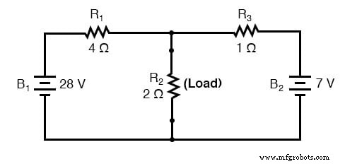
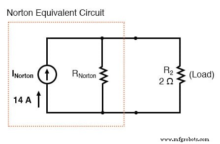
Our starting circuit and its Norton equivalent look like this:

… after applying Norton conversion …

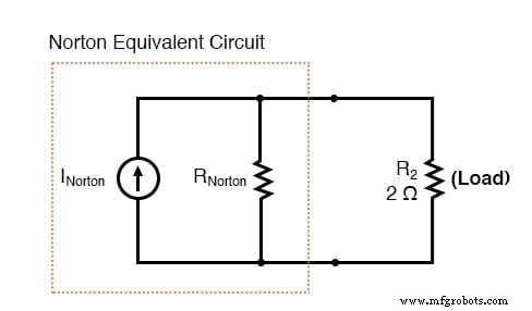
A current source delivers a fixed amount of current, providing whatever voltage is necessary to maintain that current.

Thevenin’s Theorem vs. Norton’s Theorem

Just like Thevenin’s Theorem, all elements except the load resistance are collapsed into a simpler form. The steps to compute the Norton source current (I_Norton) and Norton resistance (R_Norton) mirror those used for Thevenin’s equivalents.

Identify the Load Resistance

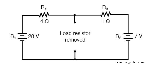
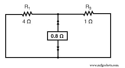
First, locate the load resistor and remove it from the original network:

Find the Norton Current

Next, short the two load terminals and calculate the resulting current. This step is the inverse of Thevenin’s approach, where the load is opened.

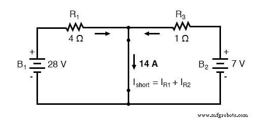
With zero voltage across the short, the current through R₁ equals the source voltage of B₁ divided by R₁: 7 A. Similarly, the current through R₃ equals the voltage of B₂ divided by R₃: 7 A. The total current through the short is 7 A + 7 A = 14 A, which becomes I_Norton in the equivalent model:

Find the Norton Resistance

To determine R_Norton, replace all independent voltage sources with short circuits and all independent current sources with opens, then measure the resistance between the two load terminals:

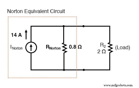
The Norton equivalent now appears as:

Compute Voltage Across the Load Resistor

Re‑attach the 2 Ω load and treat the Norton circuit as a simple parallel arrangement:

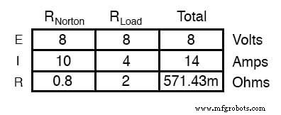
As with Thevenin’s model, the key outcome is the voltage and current across the load resistor. The Norton representation allows rapid re‑analysis for multiple load values using only basic parallel‑circuit formulas.

Review

• Norton’s Theorem reduces any linear network to a current source in parallel with a resistance, simplifying analysis of the load.
• Procedure:
  • Determine I_Norton by shorting the load and measuring the resulting current.
  • Determine R_Norton by shorting voltage sources, opening current sources, and measuring resistance between the load terminals.
  • Draw the Norton equivalent with the current source and parallel resistance, then reconnect the load.
  • Apply parallel‑circuit rules to find load voltage and current.

Related Worksheet

• Thevenin’s, Norton’s, and Maximum Power Transfer Theorems Worksheet