Precision Op‑Amp Integrator Lab: Bias‑Current Compensation & Analog Computation

PARTS AND MATERIALS

• Four 6‑volt batteries
• Operational amplifier (model 1458, Radio Shack catalog #276‑038)
• 10 kΩ linear‑taper potentiometer (Radio Shack #271‑1715)
• Two 0.1 µF non‑polarized capacitors (Radio Shack #272‑135)
• Two 100 kΩ resistors
• Three 1 MΩ resistors

 

Any modern op‑amp will run this integrator, but the LM1458 is chosen here because its high input bias current magnifies the effects you’ll learn to counteract. Although high bias currents are generally undesirable in precision circuits, they serve an educational purpose in this demonstration.

 

CROSS‑REFERENCES

Lessons in Electric Circuits, Volume 3, Chapter 8: “Operational Amplifiers”.

 

LEARNING OBJECTIVES

• Demonstrate a technique for limiting a potentiometer’s effective span.
• Explain the functional role of an integrator in signal processing.
• Illustrate how to compensate for op‑amp bias currents.

 

SCHEMATIC DIAGRAM

 

 

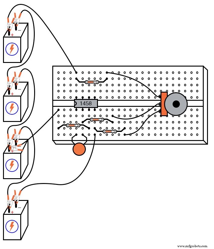
ILLUSTRATION

 

 

INSTRUCTIONS

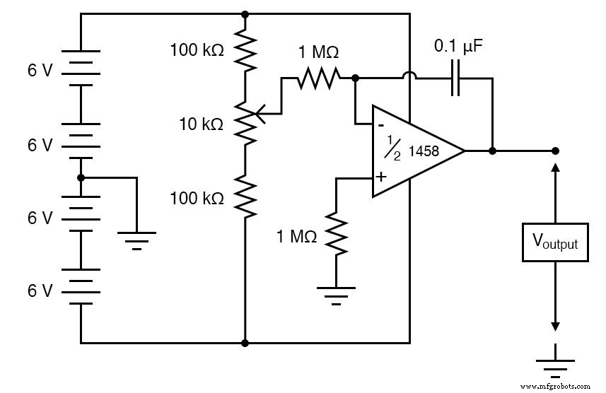
The schematic shows the potentiometer tied to the supply rails through two 100 kΩ resistors. This configuration limits the potentiometer’s output range, ensuring that a full wheel turn yields only a modest ±0.5 V swing relative to the mid‑rail reference.

When the wiper is at the far left, the output voltage is approximately +0.5 V; at the far right, it is ≈ –0.5 V. A centered wiper gives a zero‑voltage reference.

Attach a voltmeter between the op‑amp output and the circuit ground. Slowly sweep the potentiometer while observing the output voltage. The output should change at a rate set by the wiper’s deviation from center—effectively integrating the input signal over time.

With a second meter, you can simultaneously display the wiper voltage (input) and the output voltage, making the input‑to‑rate relationship visible.

Setting the potentiometer to produce zero volts should minimise the output’s rate of change. Moving away from the zero point increases the ramp slope.

Try adding the second 0.1 µF capacitor in parallel with the first. Doubling the capacitance in the feedback loop slows the integration rate, lengthening the ramp for a given wiper position.

Adding a fourth 1 MΩ resistor in parallel with the input resistor halves the effective input resistance, speeding up the integration. These variations help illustrate how component values influence the integrator’s time constant.

Integrators are foundational elements of analog computers. When combined with amplifiers, summing junctions, and variable dividers, they can model almost any linear differential equation, allowing engineers to solve equations by observing voltage levels.

Historically, analog computers simulated complex phenomena such as vehicle dynamics, rocket trajectories, and control‑system responses before digital systems emerged. While largely superseded, the constituent circuits remain valuable educational tools for visualising calculus concepts.

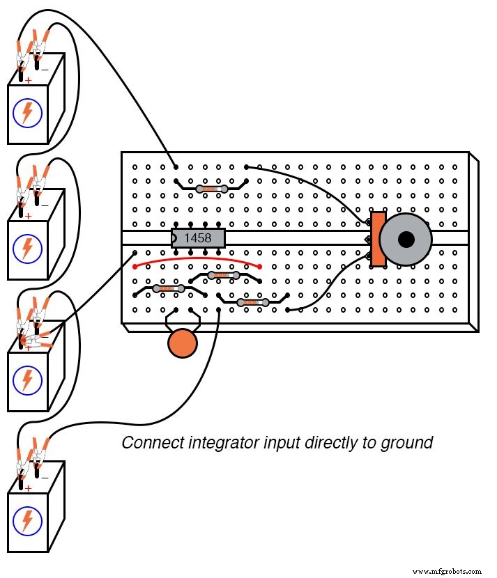
Next, move the potentiometer until the output voltage is as close to zero as possible, then disconnect the input and short the inverting terminal to ground as shown:

 

 

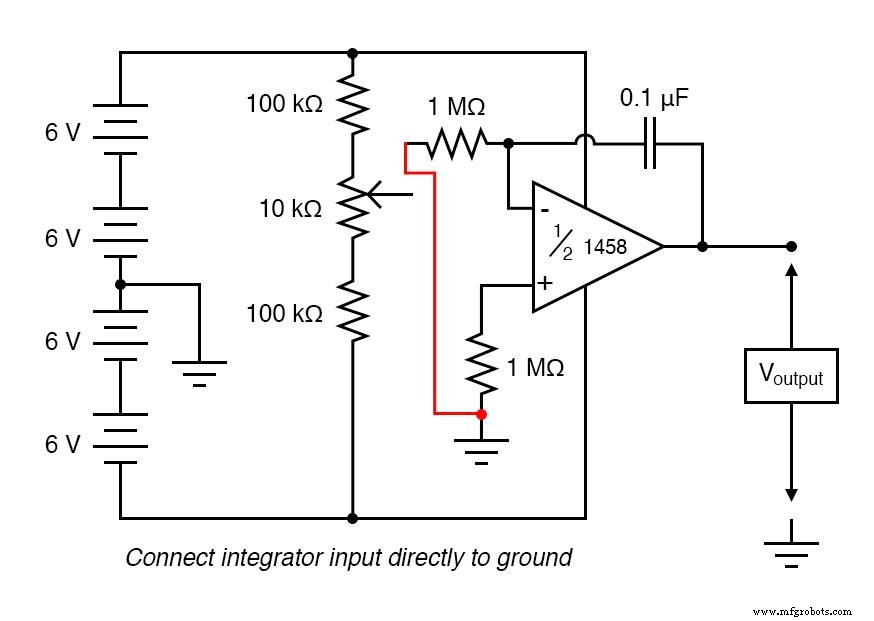
With an exact zero input, the integrator’s output should ideally remain constant. In practice, you’ll notice the output drifts slowly because real op‑amps possess tiny bias currents that flow into each input.

Short the 1 MΩ resistor that grounds the non‑inverting input. This “compensating resistor” matches the bias‑current path on both inputs, cancelling the offset voltage that would otherwise be integrated. When the resistor is bypassed, the output begins to drift; reconnecting it restores stability.

After restoring the compensating resistor, the output may still drift slightly due to the op‑amp’s bias‑voltage error, an advanced topic beyond this lab.

 

COMPUTER SIMULATION

SPICE schematic with node numbers

 

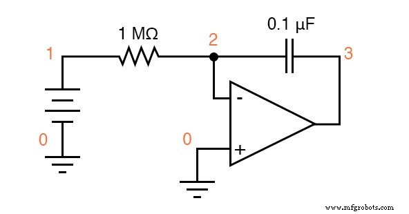
Netlist (copy the text below into a .cir file):

DC integrator vinput 1 0 dc 0.05 r1 1 2 1meg c1 2 3 0.1u ic=0 e1 3 0 0 2 999k .tran 1 30 uic .plot tran v(1,0) v(3,0) .end

 

RELATED WORKSHEETS

• AC Negative Feedback Op‑Amp Circuits Worksheet
• Linear Computational Circuitry Worksheet